User login
The ability to read and correctly interpret research is an essential skill, but most hospitalists—and physicians in general—do not receive formal training in biostatistics during their medical education.1-3 In addition to straightforward statistical tests that compare a single exposure and outcome, researchers commonly use statistical models to identify and quantify complex relationships among many exposures (eg, demographics, clinical characteristics, interventions, or other variables) and an outcome. Understanding statistical models can be challenging. Still, it is important to recognize the advantages and limitations of statistical models, how to interpret their results, and the potential implications of findings on current clinical practice.
In the article “Rates and Characteristics of Medical Malpractice Claims Against Hospitalists” published in the July 2021 issue of the Journal of Hospital Medicine, Schaffer et al4 used the Comparative Benchmarking System database, which is maintained by a malpractice insurer, to characterize malpractice claims against hospitalists. The authors used multiple logistic regression models to understand the relationship among clinical factors and indemnity payments. In this Progress Note, we describe situations in which logistic regression is the proper statistical method to analyze a data set, explain results from logistic regression analyses, and equip readers with skills to critically appraise conclusions drawn from these models.
Choosing an Appropriate Statistical Model
Statistical models often are used to describe the relationship among one or more exposure variables (ie, independent variables) and an outcome (ie, dependent variable). These models allow researchers to evaluate the effects of multiple exposure variables simultaneously, which in turn allows them to “isolate” the effect of each variable; in other words, models facilitate an understanding of the relationship between each exposure variable and the outcome, adjusted for (ie, independent of) the other exposure variables in the model.
Several statistical models can be used to quantify relationships within the data, but each type of model has certain assumptions that must be satisfied. Two important assumptions include characteristics of the outcome (eg, the type and distribution) and the nature of the relationships among the outcome and independent variables (eg, linear vs nonlinear). Simple linear regression, one of the most basic statistical models used in research,5 assumes that (a) the outcome is continuous (ie, any numeric value is possible) and normally distributed (ie, its histogram is a bell-shaped curve) and (b) the relationship between the independent variable and the outcome is linear (ie, follows a straight line). If an investigator wanted to understand how weight is related to height, a simple linear regression could be used to develop a mathematical equation that tells us how the outcome (weight) generally increases as the independent variable (height) increases.
Often, the outcome in a study is not a continuous variable but a simple success/failure variable (ie, dichotomous variable that can be one of two possible values). Schaffer et al4 examined the binary outcome of whether a malpractice claim case would end in an indemnity payment or no payment. Linear regression models are not equipped to handle dichotomous outcomes. Instead, we need to use a different statistical model: logistic regression. In logistic regression, the probability (p) of a defined outcome event is estimated by creating a regression model.
The Logistic Model
A probability (p) is a measure of how likely an event (eg, a malpractice claim ends in an indemnity payment or not) is to occur. It is always between 0 (ie, the event will definitely not occur) and 1 (ie, the event will definitely occur). A p of 0.5 means there is a 50/50 chance that the event will occur (ie, equivalent to a coin flip). Because p is a probability, we need to make sure it is always between 0 and 1. If we were to try to model p with a linear regression, the model would assume that p could extend beyond 0 and 1. What can we do?
Applying a transformation is a commonly used tool in statistics to make data work better within statistical models.6 In this case, we will transform the variable p. In logistic regression, we model the probability of experiencing the outcome through a transformation called a logit. The logit represents the natural logarithm (ln) of the ratio of the probability of experiencing the outcome (p) vs the probability of not experiencing the outcome (1 – p), with the ratio being the odds of the event occurring.

This transformation works well for dichotomous outcomes because the logit transformation approximates a straight line as long as p is not too large or too small (between 0.05 and 0.95).
If we are performing a logistic regression with only one independent variable (x) and want to understand the relationship between this variable (x) and the probability of an outcome event (p), then our model is the equation of a line. The equation for the base model of logistic regression with one independent variable (x) is

where β0 is the y-intercept and β1 is the slope of the line. Equation (2) is identical to the algebraic equation y = mx + b for a line, just rearranged slightly. In this algebraic equation, m is the slope (the same as β1) and b is the y-intercept (the same as β0). We will see that β0 and β1 are estimated (ie, assigned numeric values) from the data collected to help us understand how x and

are related and are the basis for estimating odds ratios.
We can build more complex models using multivariable logistic regression by adding more independent variables to the right side of equation (2). Essentially, this is what S
There are two notable techniques used frequently with multivariable logistic regression models. The first involves choosing which independent variables to include in the model. One way to select variables for multivariable models is defining them a priori, that is deciding which variables are clinically or conceptually associated with the outcome before looking at the data. With this approach, we can test specific hypotheses about the relationships between the independent variables and the outcome. Another common approach is to look at the data and identify the variables that vary significantly between the two outcome groups. Schaffer et al4 used an a priori approach to define variables in their multivariable model (ie, “variables for inclusion into the multivariable model were determined a priori”).
A second technique is the evaluation of collinearity, which helps us understand whether the i
Understanding the Results of the Logistic Model
Fitting the model is the process by which statistical software (eg, SAS, Stata, R, SPSS) estimates the relationships among independent variables in the model and the outcome within a specific dataset. In equation (2), this essentially means that the software will evaluate the data and provide us with the best estimates for β0 (the y-intercept) and β1 (the slope) that describe the relationship between the variable x and

Modeling can be iterative, and part of the process may include removing variables from the model that are not significantly associated with the outcome to create a simpler solution, a process known as model reduction. The results from models describe the independent association between a specific characteristic and the outcome, meaning that the relationship has been adjusted for all the other characteristics in the model.
The relationships among the independent variables and outcome are most often represented as an odds ratio (OR), which quantifies the strength of the association between two variables and is directly calculated from the β values in the model. As the name suggests, an OR is a ratio of odds. But what are odds? Simply, the odds of an outcome (such as mortality) is the probability of experiencing the event divided by the probability of not experiencing that event; in other words, it is the ratio:

The concept of odds is often unfamiliar, so it can be helpful to consider the definition in the context of games of chance. For example, in horse race betting, the outcome of interest is that a horse will lose a race. Imagine that the probability of a horse losing a race is 0.8 and the probability of winning is 0.2. The odds of losing are
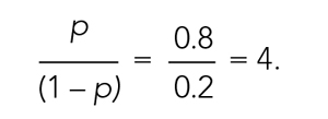
These odds usually are listed as 4-to-1, meaning that out of 5 races (ie, 4 + 1) the horse is expected to lose 4 times and win once. When odds are listed this way, we can easily calculate the associated probability by recognizing that the total number of expected races is the sum of two numbers (probability of losing: 4 races out of 5, or 0.80 vs probability of winning: 1 race out of 5, or 0.20).
In medical research, the OR typically represents the odds for one group of patients (A) compared with the odds for another group of patients (B) experiencing an outcome. If the odds of the outcome are the same for group A and group B, then OR = 1.0, meaning that the probability of the outcome is the same between the two groups. If the patients in group A have greater odds of experiencing the outcome compared with group B patients (and a greater probability of the outcome), then the OR will be >1. If the opposite is true, then the OR will be <1.
Schaffer et al4 estimated that the OR of an indemnity payment in malpractice cases involving errors in clinical judgment as a contributing factor was 5.01 (95% CI, 3.37-7.45). This means that malpractice cases involving errors in clinical judgement had a 5.01 times greater odds of indemnity payment compared with those without these errors after adjusting for all other variables in the model (eg, age, severity). Note that the 95% CI does not include 1.0. This indicates that the OR is statistically >1, and we can conclude that there is a significant relationship between errors in clinical judgment and payment that is unlikely to be attributed to chance alone.
In logistic regression for categorical independent variables, all categories are compared with a reference group within that variable, with the reference group serving as the denominator of the OR. The authors4 did not incorporate continuous independent variables in their multivariable logistic regression model. However, if the authors examined length of hospitalization as a contributing factor in indemnity payments, for example, the OR would represent a 1-unit increase in this variable (eg, 1-day increase in length of stay).
Conclusion
Logistic regression describes the relationships in data and is an important statistical model across many types of research. This Progress Note emphasizes the importance of weighing the advantages and limitations of logistic regression, provides a common approach to data transformation, and guides the correct interpretation of logistic regression model results.
1. Windish DM, Huot SJ, Green ML. Medicine residents’ understanding of the biostatistics and results in the medical literature. JAMA. 2007;298(9):1010. https://doi.org/10.1001/jama.298.9.1010
2. MacDougall M, Cameron HS, Maxwell SRJ. Medical graduate views on statistical learning needs for clinical practice: a comprehensive survey. BMC Med Educ. 2019;20(1):1. https://doi.org/10.1186/s12909-019-1842-1
3. Montori VM. Progress in evidence-based medicine. JAMA. 2008;300(15):1814-1816. https://doi.org/10.1001/jama.300.15.1814
4. Schaffer AC, Yu-Moe CW, Babayan A, Wachter RM, Einbinder JS. Rates and characteristics of medical malpractice claims against hospitalists. J Hosp Med. 2021;16(7):390-396. https://doi.org/10.12788/jhm.3557
5. Lane DM, Scott D, Hebl M, Guerra R, Osherson D, Zimmer H. Introducton to Statistics. Accessed April 13, 2021. https://onlinestatbook.com/Online_Statistics_Education.pdf
6. Marill KA. Advanced statistics: linear regression, part II: multiple linear regression. Acad Emerg Med Off J Soc Acad Emerg Med. 2004;11(1):94-102. https://doi.org/10.1197/j.aem.2003.09.006
The ability to read and correctly interpret research is an essential skill, but most hospitalists—and physicians in general—do not receive formal training in biostatistics during their medical education.1-3 In addition to straightforward statistical tests that compare a single exposure and outcome, researchers commonly use statistical models to identify and quantify complex relationships among many exposures (eg, demographics, clinical characteristics, interventions, or other variables) and an outcome. Understanding statistical models can be challenging. Still, it is important to recognize the advantages and limitations of statistical models, how to interpret their results, and the potential implications of findings on current clinical practice.
In the article “Rates and Characteristics of Medical Malpractice Claims Against Hospitalists” published in the July 2021 issue of the Journal of Hospital Medicine, Schaffer et al4 used the Comparative Benchmarking System database, which is maintained by a malpractice insurer, to characterize malpractice claims against hospitalists. The authors used multiple logistic regression models to understand the relationship among clinical factors and indemnity payments. In this Progress Note, we describe situations in which logistic regression is the proper statistical method to analyze a data set, explain results from logistic regression analyses, and equip readers with skills to critically appraise conclusions drawn from these models.
Choosing an Appropriate Statistical Model
Statistical models often are used to describe the relationship among one or more exposure variables (ie, independent variables) and an outcome (ie, dependent variable). These models allow researchers to evaluate the effects of multiple exposure variables simultaneously, which in turn allows them to “isolate” the effect of each variable; in other words, models facilitate an understanding of the relationship between each exposure variable and the outcome, adjusted for (ie, independent of) the other exposure variables in the model.
Several statistical models can be used to quantify relationships within the data, but each type of model has certain assumptions that must be satisfied. Two important assumptions include characteristics of the outcome (eg, the type and distribution) and the nature of the relationships among the outcome and independent variables (eg, linear vs nonlinear). Simple linear regression, one of the most basic statistical models used in research,5 assumes that (a) the outcome is continuous (ie, any numeric value is possible) and normally distributed (ie, its histogram is a bell-shaped curve) and (b) the relationship between the independent variable and the outcome is linear (ie, follows a straight line). If an investigator wanted to understand how weight is related to height, a simple linear regression could be used to develop a mathematical equation that tells us how the outcome (weight) generally increases as the independent variable (height) increases.
Often, the outcome in a study is not a continuous variable but a simple success/failure variable (ie, dichotomous variable that can be one of two possible values). Schaffer et al4 examined the binary outcome of whether a malpractice claim case would end in an indemnity payment or no payment. Linear regression models are not equipped to handle dichotomous outcomes. Instead, we need to use a different statistical model: logistic regression. In logistic regression, the probability (p) of a defined outcome event is estimated by creating a regression model.
The Logistic Model
A probability (p) is a measure of how likely an event (eg, a malpractice claim ends in an indemnity payment or not) is to occur. It is always between 0 (ie, the event will definitely not occur) and 1 (ie, the event will definitely occur). A p of 0.5 means there is a 50/50 chance that the event will occur (ie, equivalent to a coin flip). Because p is a probability, we need to make sure it is always between 0 and 1. If we were to try to model p with a linear regression, the model would assume that p could extend beyond 0 and 1. What can we do?
Applying a transformation is a commonly used tool in statistics to make data work better within statistical models.6 In this case, we will transform the variable p. In logistic regression, we model the probability of experiencing the outcome through a transformation called a logit. The logit represents the natural logarithm (ln) of the ratio of the probability of experiencing the outcome (p) vs the probability of not experiencing the outcome (1 – p), with the ratio being the odds of the event occurring.
This transformation works well for dichotomous outcomes because the logit transformation approximates a straight line as long as p is not too large or too small (between 0.05 and 0.95).
If we are performing a logistic regression with only one independent variable (x) and want to understand the relationship between this variable (x) and the probability of an outcome event (p), then our model is the equation of a line. The equation for the base model of logistic regression with one independent variable (x) is
where β0 is the y-intercept and β1 is the slope of the line. Equation (2) is identical to the algebraic equation y = mx + b for a line, just rearranged slightly. In this algebraic equation, m is the slope (the same as β1) and b is the y-intercept (the same as β0). We will see that β0 and β1 are estimated (ie, assigned numeric values) from the data collected to help us understand how x and
are related and are the basis for estimating odds ratios.
We can build more complex models using multivariable logistic regression by adding more independent variables to the right side of equation (2). Essentially, this is what S
There are two notable techniques used frequently with multivariable logistic regression models. The first involves choosing which independent variables to include in the model. One way to select variables for multivariable models is defining them a priori, that is deciding which variables are clinically or conceptually associated with the outcome before looking at the data. With this approach, we can test specific hypotheses about the relationships between the independent variables and the outcome. Another common approach is to look at the data and identify the variables that vary significantly between the two outcome groups. Schaffer et al4 used an a priori approach to define variables in their multivariable model (ie, “variables for inclusion into the multivariable model were determined a priori”).
A second technique is the evaluation of collinearity, which helps us understand whether the i
Understanding the Results of the Logistic Model
Fitting the model is the process by which statistical software (eg, SAS, Stata, R, SPSS) estimates the relationships among independent variables in the model and the outcome within a specific dataset. In equation (2), this essentially means that the software will evaluate the data and provide us with the best estimates for β0 (the y-intercept) and β1 (the slope) that describe the relationship between the variable x and
Modeling can be iterative, and part of the process may include removing variables from the model that are not significantly associated with the outcome to create a simpler solution, a process known as model reduction. The results from models describe the independent association between a specific characteristic and the outcome, meaning that the relationship has been adjusted for all the other characteristics in the model.
The relationships among the independent variables and outcome are most often represented as an odds ratio (OR), which quantifies the strength of the association between two variables and is directly calculated from the β values in the model. As the name suggests, an OR is a ratio of odds. But what are odds? Simply, the odds of an outcome (such as mortality) is the probability of experiencing the event divided by the probability of not experiencing that event; in other words, it is the ratio:
The concept of odds is often unfamiliar, so it can be helpful to consider the definition in the context of games of chance. For example, in horse race betting, the outcome of interest is that a horse will lose a race. Imagine that the probability of a horse losing a race is 0.8 and the probability of winning is 0.2. The odds of losing are
These odds usually are listed as 4-to-1, meaning that out of 5 races (ie, 4 + 1) the horse is expected to lose 4 times and win once. When odds are listed this way, we can easily calculate the associated probability by recognizing that the total number of expected races is the sum of two numbers (probability of losing: 4 races out of 5, or 0.80 vs probability of winning: 1 race out of 5, or 0.20).
In medical research, the OR typically represents the odds for one group of patients (A) compared with the odds for another group of patients (B) experiencing an outcome. If the odds of the outcome are the same for group A and group B, then OR = 1.0, meaning that the probability of the outcome is the same between the two groups. If the patients in group A have greater odds of experiencing the outcome compared with group B patients (and a greater probability of the outcome), then the OR will be >1. If the opposite is true, then the OR will be <1.
Schaffer et al4 estimated that the OR of an indemnity payment in malpractice cases involving errors in clinical judgment as a contributing factor was 5.01 (95% CI, 3.37-7.45). This means that malpractice cases involving errors in clinical judgement had a 5.01 times greater odds of indemnity payment compared with those without these errors after adjusting for all other variables in the model (eg, age, severity). Note that the 95% CI does not include 1.0. This indicates that the OR is statistically >1, and we can conclude that there is a significant relationship between errors in clinical judgment and payment that is unlikely to be attributed to chance alone.
In logistic regression for categorical independent variables, all categories are compared with a reference group within that variable, with the reference group serving as the denominator of the OR. The authors4 did not incorporate continuous independent variables in their multivariable logistic regression model. However, if the authors examined length of hospitalization as a contributing factor in indemnity payments, for example, the OR would represent a 1-unit increase in this variable (eg, 1-day increase in length of stay).
Conclusion
Logistic regression describes the relationships in data and is an important statistical model across many types of research. This Progress Note emphasizes the importance of weighing the advantages and limitations of logistic regression, provides a common approach to data transformation, and guides the correct interpretation of logistic regression model results.
1. Windish DM, Huot SJ, Green ML. Medicine residents’ understanding of the biostatistics and results in the medical literature. JAMA. 2007;298(9):1010. https://doi.org/10.1001/jama.298.9.1010
2. MacDougall M, Cameron HS, Maxwell SRJ. Medical graduate views on statistical learning needs for clinical practice: a comprehensive survey. BMC Med Educ. 2019;20(1):1. https://doi.org/10.1186/s12909-019-1842-1
3. Montori VM. Progress in evidence-based medicine. JAMA. 2008;300(15):1814-1816. https://doi.org/10.1001/jama.300.15.1814
4. Schaffer AC, Yu-Moe CW, Babayan A, Wachter RM, Einbinder JS. Rates and characteristics of medical malpractice claims against hospitalists. J Hosp Med. 2021;16(7):390-396. https://doi.org/10.12788/jhm.3557
5. Lane DM, Scott D, Hebl M, Guerra R, Osherson D, Zimmer H. Introducton to Statistics. Accessed April 13, 2021. https://onlinestatbook.com/Online_Statistics_Education.pdf
6. Marill KA. Advanced statistics: linear regression, part II: multiple linear regression. Acad Emerg Med Off J Soc Acad Emerg Med. 2004;11(1):94-102. https://doi.org/10.1197/j.aem.2003.09.006
© 2021 Society of Hospital Medicine