User login
Regional Variation in Standardized Costs of Care at Children’s Hospitals
With some areas of the country spending close to 3 times more on healthcare than others, regional variation in healthcare spending has been the focus of national attention.1-7 Since 1973, the Dartmouth Institute has studied regional variation in healthcare utilization and spending and concluded that variation is “unwarranted” because it is driven by providers’ practice patterns rather than differences in medical need, patient preferences, or evidence-based medicine.8-11 However, critics of the Dartmouth Institute’s findings argue that their approach does not adequately adjust for community-level income, and that higher costs in some areas reflect greater patient needs that are not reflected in illness acuity alone.12-14
While Medicare data have made it possible to study variations in spending for the senior population, fragmentation of insurance coverage and nonstandardized data structures make studying the pediatric population more difficult. However, the Children’s Hospital Association’s (CHA) Pediatric Health Information System (PHIS) has made large-scale comparisons more feasible. To overcome challenges associated with using charges and nonuniform cost data, PHIS-derived standardized costs provide new opportunities for comparisons.15,16 Initial analyses using PHIS data showed significant interhospital variations in costs of care,15 but they did not adjust for differences in populations and assess the drivers of variation. A more recent study that controlled for payer status, comorbidities, and illness severity found that intensive care unit (ICU) utilization varied significantly for children hospitalized for asthma, suggesting that hospital practice patterns drive differences in cost.17
This study uses PHIS data to analyze regional variations in standardized costs of care for 3 conditions for which children are hospitalized. To assess potential drivers of variation, the study investigates the effects of patient-level demographic and illness-severity variables as well as encounter-level variables on costs of care. It also estimates cost savings from reducing variation.
METHODS
Data Source
This retrospective cohort study uses the PHIS database (CHA, Overland Park, KS), which includes 48 freestanding children’s hospitals located in noncompeting markets across the United States and accounts for approximately 20% of pediatric hospitalizations. PHIS includes patient demographics, International Classification of Diseases, 9th Revision (ICD-9) diagnosis and procedure codes, as well as hospital charges. In addition to total charges, PHIS reports imaging, laboratory, pharmacy, and “other” charges. The “other” category aggregates clinical, supply, room, and nursing charges (including facility fees and ancillary staff services).
Inclusion Criteria
Inpatient- and observation-status hospitalizations for asthma, diabetic ketoacidosis (DKA), and acute gastroenteritis (AGE) at 46 PHIS hospitals from October 2014 to September 2015 were included. Two hospitals were excluded because of missing data. Hospitalizations for patients >18 years were excluded.
Hospitalizations were categorized by using All Patient Refined-Diagnosis Related Groups (APR-DRGs) version 24 (3M Health Information Systems, St. Paul, MN)18 based on the ICD-9 diagnosis and procedure codes assigned during the episode of care. Analyses included APR-DRG 141 (asthma), primary diagnosis ICD-9 codes 250.11 and 250.13 (DKA), and APR-DRG 249 (AGE). ICD-9 codes were used for DKA for increased specificity.19 These conditions were chosen to represent 3 clinical scenarios: (1) a diagnosis for which hospitals differ on whether certain aspects of care are provided in the ICU (asthma), (2) a diagnosis that frequently includes care in an ICU (DKA), and (3) a diagnosis that typically does not include ICU care (AGE).19
Study Design
To focus the analysis on variation in resource utilization across hospitals rather than variations in hospital item charges, each billed resource was assigned a standardized cost.15,16 For each clinical transaction code (CTC), the median unit cost was calculated for each hospital. The median of the hospital medians was defined as the standardized unit cost for that CTC.
The primary outcome variable was the total standardized cost for the hospitalization adjusted for patient-level demographic and illness-severity variables. Patient demographic and illness-severity covariates included age, race, gender, ZIP code-based median annual household income (HHI), rural-urban location, distance from home ZIP code to the hospital, chronic condition indicator (CCI), and severity-of-illness (SOI). When assessing drivers of variation, encounter-level covariates were added, including length of stay (LOS) in hours, ICU utilization, and 7-day readmission (an imprecise measure to account for quality of care during the index visit). The contribution of imaging, laboratory, pharmacy, and “other” costs was also considered.
Median annual HHI for patients’ home ZIP code was obtained from 2010 US Census data. Community-level HHI, a proxy for socioeconomic status (SES),20,21 was classified into categories based on the 2015 US federal poverty level (FPL) for a family of 422: HHI-1 = ≤ 1.5 × FPL; HHI-2 = 1.5 to 2 × FPL; HHI-3 = 2 to 3 × FPL; HHI-4 = ≥ 3 × FPL. Rural-urban commuting area (RUCA) codes were used to determine the rural-urban classification of the patient’s home.23 The distance from home ZIP code to the hospital was included as an additional control for illness severity because patients traveling longer distances are often more sick and require more resources.24
The Agency for Healthcare Research and Quality CCI classification system was used to identify the presence of a chronic condition.25 For asthma, CCI was flagged if the patient had a chronic condition other than asthma; for DKA, CCI was flagged if the patient had a chronic condition other than DKA; and for AGE, CCI was flagged if the patient had any chronic condition.
The APR-DRG system provides a 4-level SOI score with each APR-DRG category. Patient factors, such as comorbid diagnoses, are considered in severity scores generated through 3M’s proprietary algorithms.18
For the first analysis, the 46 hospitals were categorized into 7 geographic regions based on 2010 US Census Divisions.26 To overcome small hospital sample sizes, Mountain and Pacific were combined into West, and Middle Atlantic and New England were combined into North East. Because PHIS hospitals are located in noncompeting geographic regions, for the second analysis, we examined hospital-level variation (considering each hospital as its own region).
Data Analysis
To focus the analysis on “typical” patients and produce more robust estimates of central tendencies, the top and bottom 5% of hospitalizations with the most extreme standardized costs by condition were trimmed.27 Standardized costs were log-transformed because of their nonnormal distribution and analyzed by using linear mixed models. Covariates were added stepwise to assess the proportion of the variance explained by each predictor. Post-hoc tests with conservative single-step stepwise mutation model corrections for multiple testing were used to compare adjusted costs. Statistical analyses were performed using SAS version 9.3 (SAS Institute, Cary, NC). P values < 0.05 were considered significant. The Children’s Hospital of Philadelphia Institutional Review Board did not classify this study as human subjects research.
RESULTS

During the study period, there were 26,430 hospitalizations for asthma, 5056 for DKA, and 16,274 for AGE (Table 1).
Variation Across Census Regions
After adjusting for patient-level demographic and illness-severity variables, differences in adjusted total standardized costs remained between regions (P < 0.001). Although no region was an outlier compared to the overall mean for any of the conditions, regions were statistically different in pairwise comparison. The East North Central, South Atlantic, and West South Central regions had the highest adjusted total standardized costs for each of the conditions. The East South Central and West North Central regions had the lowest costs for each of the conditions. Adjusted total standardized costs were 120% higher for asthma ($1920 vs $4227), 46% higher for DKA ($7429 vs $10,881), and 150% higher for AGE ($3316 vs $8292) in the highest-cost region compared with the lowest-cost region (Table 2A).
Variation Within Census Regions

After controlling for patient-level demographic and illness-severity variables, standardized costs were different across hospitals in the same region (P < 0.001; panel A in Figure). This was true for all conditions in each region. Differences between the lowest- and highest-cost hospitals within the same region ranged from 111% to 420% for asthma, 101% to 398% for DKA, and 166% to 787% for AGE (Table 3).
Variation Across Hospitals (Each Hospital as Its Own Region)
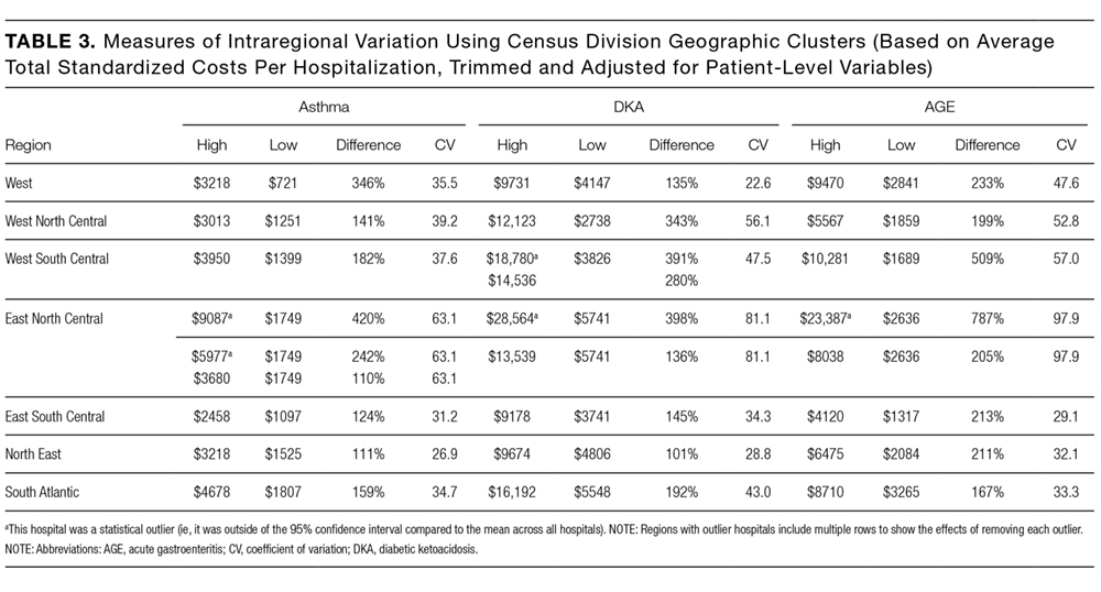
One hospital had the highest adjusted standardized costs for all 3 conditions ($9087 for asthma, $28,564 for DKA, and $23,387 for AGE) and was outside of the 95% confidence interval compared with the overall means. The second highest-cost hospitals for asthma ($5977) and AGE ($18,780) were also outside of the 95% confidence interval. After removing these outliers, the difference between the highest- and lowest-cost hospitals was 549% for asthma ($721 vs $4678), 491% for DKA ($2738 vs $16,192), and 681% for AGE ($1317 vs $10,281; Table 2B).
Drivers of Variation Across Census Regions
Patient-level demographic and illness-severity variables explained very little of the variation in standardized costs across regions. For each of the conditions, age, race, gender, community-level HHI, RUCA, and distance from home to the hospital each accounted for <1.5% of variation, while SOI and CCI each accounted for <5%. Overall, patient-level variables explained 5.5%, 3.7%, and 6.7% of variation for asthma, DKA, and AGE.
Encounter-level variables explained a much larger percentage of the variation in costs. LOS accounted for 17.8% of the variation for asthma, 9.8% for DKA, and 8.7% for AGE. ICU utilization explained 6.9% of the variation for asthma and 12.5% for DKA; ICU use was not a major driver for AGE. Seven-day readmissions accounted for <0.5% for each of the conditions. The combination of patient-level and encounter-level variables explained 27%, 24%, and 15% of the variation for asthma, DKA, and AGE.
Drivers of Variation Across Hospitals
For each of the conditions, patient-level demographic variables each accounted for <2% of variation in costs between hospitals. SOI accounted for 4.5% of the variation for asthma and CCI accounted for 5.2% for AGE. Overall, patient-level variables explained 6.9%, 5.3%, and 7.3% of variation for asthma, DKA, and AGE.
Encounter-level variables accounted for a much larger percentage of the variation in cost. LOS explained 25.4% for asthma, 13.3% for DKA, and 14.2% for AGE. ICU utilization accounted for 13.4% for asthma and 21.9% for DKA; ICU use was not a major driver for AGE. Seven-day readmissions accounted for <0.5% for each of the conditions. Together, patient-level and encounter-level variables explained 40%, 36%, and 22% of variation for asthma, DKA, and AGE.
Imaging, Laboratory, Pharmacy, and “Other” Costs
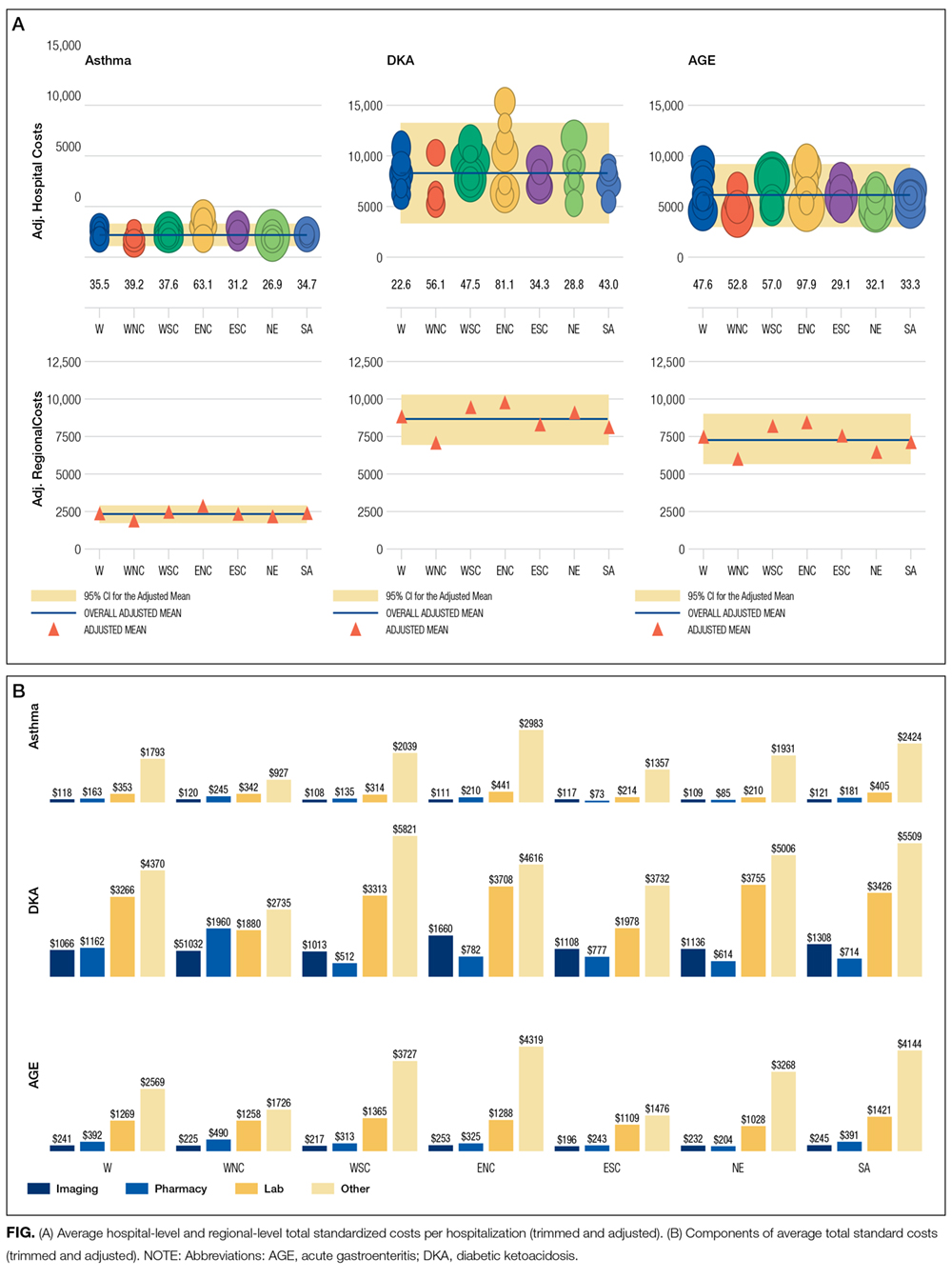
The largest contributor to total costs adjusted for patient-level factors for all conditions was “other,” which aggregates room, nursing, clinical, and supply charges (panel B in Figure). When considering drivers of variation, this category explained >50% for each of the conditions. The next largest contributor to total costs was laboratory charges, which accounted for 15% of the variation across regions for asthma and 11% for DKA. Differences in imaging accounted for 18% of the variation for DKA and 15% for AGE. Differences in pharmacy charges accounted for <4% of the variation for each of the conditions. Adding the 4 cost components to the other patient- and encounter-level covariates, the model explained 81%, 78%, and 72% of the variation across census regions for asthma, DKA, and AGE.
For the hospital-level analysis, differences in “other” remained the largest driver of cost variation. For asthma, “other” explained 61% of variation, while pharmacy, laboratory, and imaging each accounted for <8%. For DKA, differences in imaging accounted for 18% of the variation and laboratory charges accounted for 12%. For AGE, imaging accounted for 15% of the variation. Adding the 4 cost components to the other patient- and encounter-level covariates, the model explained 81%, 72%, and 67% of the variation for asthma, DKA, and AGE.
Cost Savings
If all hospitals in this cohort with adjusted standardized costs above the national PHIS average achieved costs equal to the national PHIS average, estimated annual savings in adjusted standardized costs for these 3 conditions would be $69.1 million. If each hospital with adjusted costs above the average within its census region achieved costs equal to its regional average, estimated annual savings in adjusted standardized costs for these conditions would be $25.2 million.
DISCUSSION
This study reported on the regional variation in costs of care for 3 conditions treated at 46 children’s hospitals across 7 geographic regions, and it demonstrated that variations in costs of care exist in pediatrics. This study used standardized costs to compare utilization patterns across hospitals and adjusted for several patient-level demographic and illness-severity factors, and it found that differences in costs of care for children hospitalized with asthma, DKA, and AGE remained both between and within regions.
These variations are noteworthy, as hospitals strive to improve the value of healthcare. If the higher-cost hospitals in this cohort could achieve costs equal to the national PHIS averages, estimated annual savings in adjusted standardized costs for these conditions alone would equal $69.1 million. If higher-cost hospitals relative to the average in their own region reduced costs to their regional averages, annual standardized cost savings could equal $25.2 million for these conditions.
The differences observed are also significant in that they provide a foundation for exploring whether lower-cost regions or lower-cost hospitals achieve comparable quality outcomes.28 If so, studying what those hospitals do to achieve outcomes more efficiently can serve as the basis for the establishment of best practices.29 Standardizing best practices through protocols, pathways, and care-model redesign can reduce potentially unnecessary spending.30
Our findings showed that patient-level demographic and illness-severity covariates, including community-level HHI and SOI, did not consistently explain cost differences. Instead, LOS and ICU utilization were associated with higher costs.17,19 When considering the effect of the 4 cost components on the variation in total standardized costs between regions and between hospitals, the fact that the “other” category accounted for the largest percent of the variation is not surprising, because the cost of room occupancy and nursing services increases with longer LOS and more time in the ICU. Other individual cost components that were major drivers of variation were laboratory utilization for asthma and imaging for DKA and AGE31 (though they accounted for a much smaller proportion of total adjusted costs).19
To determine if these factors are modifiable, more information is needed to explain why practices differ. Many factors may contribute to varying utilization patterns, including differences in capabilities and resources (in the hospital and in the community) and patient volumes. For example, some hospitals provide continuous albuterol for status asthmaticus only in ICUs, while others provide it on regular units.32 But if certain hospitals do not have adequate resources or volumes to effectively care for certain populations outside of the ICU, their higher-value approach (considering quality and cost) may be to utilize ICU beds, even if some other hospitals care for those patients on non-ICU floors. Another possibility is that family preferences about care delivery (such as how long children stay in the hospital) may vary across regions.33
Other evidence suggests that physician practice and spending patterns are strongly influenced by the practices of the region where they trained.34 Because physicians often practice close to where they trained,35,36 this may partially explain how regional patterns are reinforced.
Even considering all mentioned covariates, our model did not fully explain variation in standardized costs. After adding the cost components as covariates, between one-third and one-fifth of the variation remained unexplained. It is possible that this unexplained variation stemmed from unmeasured patient-level factors.
In addition, while proxies for SES, including community-level HHI, did not significantly predict differences in costs across regions, it is possible that SES affected LOS differently in different regions. Previous studies have suggested that lower SES is associated with longer LOS.37 If this effect is more pronounced in certain regions (potentially because of differences in social service infrastructures), SES may be contributing to variations in cost through LOS.
Our findings were subject to limitations. First, this study only examined 3 diagnoses and did not include surgical or less common conditions. Second, while PHIS includes tertiary care, academic, and freestanding children’s hospitals, it does not include general hospitals, which is where most pediatric patients receive care.38 Third, we used ZIP code-based median annual HHI to account for SES, and we used ZIP codes to determine the distance to the hospital and rural-urban location of patients’ homes. These approximations lack precision because SES and distances vary within ZIP codes.39 Fourth, while adjusted standardized costs allow for comparisons between hospitals, they do not represent actual costs to patients or individual hospitals. Additionally, when determining whether variation remained after controlling for patient-level variables, we included SOI as a reflection of illness-severity at presentation. However, in practice, SOI scores may be assigned partially based on factors determined during the hospitalization.18 Finally, the use of other regional boundaries or the selection of different hospitals may yield different results.
CONCLUSION
This study reveals regional variations in costs of care for 3 inpatient pediatric conditions. Future studies should explore whether lower-cost regions or lower-cost hospitals achieve comparable quality outcomes. To the extent that variation is driven by modifiable factors and lower spending does not compromise outcomes, these data may prompt reviews of care models to reduce unwarranted variation and improve the value of care delivery at local, regional, and national levels.
Disclosure
Internal funds from the CHA and The Children’s Hospital of Philadelphia supported the conduct of this work. The authors have no financial interests, relationships, or affiliations relevant to the subject matter or materials discussed in the manuscript to disclose. The authors have no potential conflicts of interest relevant to the subject matter or materials discussed in the manuscript to disclose
1. Fisher E, Skinner J. Making Sense of Geographic Variations in Health Care: The New IOM Report. 2013; http://healthaffairs.org/blog/2013/07/24/making-sense-of-geographic-variations-in-health-care-the-new-iom-report/. Accessed on April 11, 2014.
With some areas of the country spending close to 3 times more on healthcare than others, regional variation in healthcare spending has been the focus of national attention.1-7 Since 1973, the Dartmouth Institute has studied regional variation in healthcare utilization and spending and concluded that variation is “unwarranted” because it is driven by providers’ practice patterns rather than differences in medical need, patient preferences, or evidence-based medicine.8-11 However, critics of the Dartmouth Institute’s findings argue that their approach does not adequately adjust for community-level income, and that higher costs in some areas reflect greater patient needs that are not reflected in illness acuity alone.12-14
While Medicare data have made it possible to study variations in spending for the senior population, fragmentation of insurance coverage and nonstandardized data structures make studying the pediatric population more difficult. However, the Children’s Hospital Association’s (CHA) Pediatric Health Information System (PHIS) has made large-scale comparisons more feasible. To overcome challenges associated with using charges and nonuniform cost data, PHIS-derived standardized costs provide new opportunities for comparisons.15,16 Initial analyses using PHIS data showed significant interhospital variations in costs of care,15 but they did not adjust for differences in populations and assess the drivers of variation. A more recent study that controlled for payer status, comorbidities, and illness severity found that intensive care unit (ICU) utilization varied significantly for children hospitalized for asthma, suggesting that hospital practice patterns drive differences in cost.17
This study uses PHIS data to analyze regional variations in standardized costs of care for 3 conditions for which children are hospitalized. To assess potential drivers of variation, the study investigates the effects of patient-level demographic and illness-severity variables as well as encounter-level variables on costs of care. It also estimates cost savings from reducing variation.
METHODS
Data Source
This retrospective cohort study uses the PHIS database (CHA, Overland Park, KS), which includes 48 freestanding children’s hospitals located in noncompeting markets across the United States and accounts for approximately 20% of pediatric hospitalizations. PHIS includes patient demographics, International Classification of Diseases, 9th Revision (ICD-9) diagnosis and procedure codes, as well as hospital charges. In addition to total charges, PHIS reports imaging, laboratory, pharmacy, and “other” charges. The “other” category aggregates clinical, supply, room, and nursing charges (including facility fees and ancillary staff services).
Inclusion Criteria
Inpatient- and observation-status hospitalizations for asthma, diabetic ketoacidosis (DKA), and acute gastroenteritis (AGE) at 46 PHIS hospitals from October 2014 to September 2015 were included. Two hospitals were excluded because of missing data. Hospitalizations for patients >18 years were excluded.
Hospitalizations were categorized by using All Patient Refined-Diagnosis Related Groups (APR-DRGs) version 24 (3M Health Information Systems, St. Paul, MN)18 based on the ICD-9 diagnosis and procedure codes assigned during the episode of care. Analyses included APR-DRG 141 (asthma), primary diagnosis ICD-9 codes 250.11 and 250.13 (DKA), and APR-DRG 249 (AGE). ICD-9 codes were used for DKA for increased specificity.19 These conditions were chosen to represent 3 clinical scenarios: (1) a diagnosis for which hospitals differ on whether certain aspects of care are provided in the ICU (asthma), (2) a diagnosis that frequently includes care in an ICU (DKA), and (3) a diagnosis that typically does not include ICU care (AGE).19
Study Design
To focus the analysis on variation in resource utilization across hospitals rather than variations in hospital item charges, each billed resource was assigned a standardized cost.15,16 For each clinical transaction code (CTC), the median unit cost was calculated for each hospital. The median of the hospital medians was defined as the standardized unit cost for that CTC.
The primary outcome variable was the total standardized cost for the hospitalization adjusted for patient-level demographic and illness-severity variables. Patient demographic and illness-severity covariates included age, race, gender, ZIP code-based median annual household income (HHI), rural-urban location, distance from home ZIP code to the hospital, chronic condition indicator (CCI), and severity-of-illness (SOI). When assessing drivers of variation, encounter-level covariates were added, including length of stay (LOS) in hours, ICU utilization, and 7-day readmission (an imprecise measure to account for quality of care during the index visit). The contribution of imaging, laboratory, pharmacy, and “other” costs was also considered.
Median annual HHI for patients’ home ZIP code was obtained from 2010 US Census data. Community-level HHI, a proxy for socioeconomic status (SES),20,21 was classified into categories based on the 2015 US federal poverty level (FPL) for a family of 422: HHI-1 = ≤ 1.5 × FPL; HHI-2 = 1.5 to 2 × FPL; HHI-3 = 2 to 3 × FPL; HHI-4 = ≥ 3 × FPL. Rural-urban commuting area (RUCA) codes were used to determine the rural-urban classification of the patient’s home.23 The distance from home ZIP code to the hospital was included as an additional control for illness severity because patients traveling longer distances are often more sick and require more resources.24
The Agency for Healthcare Research and Quality CCI classification system was used to identify the presence of a chronic condition.25 For asthma, CCI was flagged if the patient had a chronic condition other than asthma; for DKA, CCI was flagged if the patient had a chronic condition other than DKA; and for AGE, CCI was flagged if the patient had any chronic condition.
The APR-DRG system provides a 4-level SOI score with each APR-DRG category. Patient factors, such as comorbid diagnoses, are considered in severity scores generated through 3M’s proprietary algorithms.18
For the first analysis, the 46 hospitals were categorized into 7 geographic regions based on 2010 US Census Divisions.26 To overcome small hospital sample sizes, Mountain and Pacific were combined into West, and Middle Atlantic and New England were combined into North East. Because PHIS hospitals are located in noncompeting geographic regions, for the second analysis, we examined hospital-level variation (considering each hospital as its own region).
Data Analysis
To focus the analysis on “typical” patients and produce more robust estimates of central tendencies, the top and bottom 5% of hospitalizations with the most extreme standardized costs by condition were trimmed.27 Standardized costs were log-transformed because of their nonnormal distribution and analyzed by using linear mixed models. Covariates were added stepwise to assess the proportion of the variance explained by each predictor. Post-hoc tests with conservative single-step stepwise mutation model corrections for multiple testing were used to compare adjusted costs. Statistical analyses were performed using SAS version 9.3 (SAS Institute, Cary, NC). P values < 0.05 were considered significant. The Children’s Hospital of Philadelphia Institutional Review Board did not classify this study as human subjects research.
RESULTS
During the study period, there were 26,430 hospitalizations for asthma, 5056 for DKA, and 16,274 for AGE (Table 1).
Variation Across Census Regions
After adjusting for patient-level demographic and illness-severity variables, differences in adjusted total standardized costs remained between regions (P < 0.001). Although no region was an outlier compared to the overall mean for any of the conditions, regions were statistically different in pairwise comparison. The East North Central, South Atlantic, and West South Central regions had the highest adjusted total standardized costs for each of the conditions. The East South Central and West North Central regions had the lowest costs for each of the conditions. Adjusted total standardized costs were 120% higher for asthma ($1920 vs $4227), 46% higher for DKA ($7429 vs $10,881), and 150% higher for AGE ($3316 vs $8292) in the highest-cost region compared with the lowest-cost region (Table 2A).
Variation Within Census Regions
After controlling for patient-level demographic and illness-severity variables, standardized costs were different across hospitals in the same region (P < 0.001; panel A in Figure). This was true for all conditions in each region. Differences between the lowest- and highest-cost hospitals within the same region ranged from 111% to 420% for asthma, 101% to 398% for DKA, and 166% to 787% for AGE (Table 3).
Variation Across Hospitals (Each Hospital as Its Own Region)
One hospital had the highest adjusted standardized costs for all 3 conditions ($9087 for asthma, $28,564 for DKA, and $23,387 for AGE) and was outside of the 95% confidence interval compared with the overall means. The second highest-cost hospitals for asthma ($5977) and AGE ($18,780) were also outside of the 95% confidence interval. After removing these outliers, the difference between the highest- and lowest-cost hospitals was 549% for asthma ($721 vs $4678), 491% for DKA ($2738 vs $16,192), and 681% for AGE ($1317 vs $10,281; Table 2B).
Drivers of Variation Across Census Regions
Patient-level demographic and illness-severity variables explained very little of the variation in standardized costs across regions. For each of the conditions, age, race, gender, community-level HHI, RUCA, and distance from home to the hospital each accounted for <1.5% of variation, while SOI and CCI each accounted for <5%. Overall, patient-level variables explained 5.5%, 3.7%, and 6.7% of variation for asthma, DKA, and AGE.
Encounter-level variables explained a much larger percentage of the variation in costs. LOS accounted for 17.8% of the variation for asthma, 9.8% for DKA, and 8.7% for AGE. ICU utilization explained 6.9% of the variation for asthma and 12.5% for DKA; ICU use was not a major driver for AGE. Seven-day readmissions accounted for <0.5% for each of the conditions. The combination of patient-level and encounter-level variables explained 27%, 24%, and 15% of the variation for asthma, DKA, and AGE.
Drivers of Variation Across Hospitals
For each of the conditions, patient-level demographic variables each accounted for <2% of variation in costs between hospitals. SOI accounted for 4.5% of the variation for asthma and CCI accounted for 5.2% for AGE. Overall, patient-level variables explained 6.9%, 5.3%, and 7.3% of variation for asthma, DKA, and AGE.
Encounter-level variables accounted for a much larger percentage of the variation in cost. LOS explained 25.4% for asthma, 13.3% for DKA, and 14.2% for AGE. ICU utilization accounted for 13.4% for asthma and 21.9% for DKA; ICU use was not a major driver for AGE. Seven-day readmissions accounted for <0.5% for each of the conditions. Together, patient-level and encounter-level variables explained 40%, 36%, and 22% of variation for asthma, DKA, and AGE.
Imaging, Laboratory, Pharmacy, and “Other” Costs
The largest contributor to total costs adjusted for patient-level factors for all conditions was “other,” which aggregates room, nursing, clinical, and supply charges (panel B in Figure). When considering drivers of variation, this category explained >50% for each of the conditions. The next largest contributor to total costs was laboratory charges, which accounted for 15% of the variation across regions for asthma and 11% for DKA. Differences in imaging accounted for 18% of the variation for DKA and 15% for AGE. Differences in pharmacy charges accounted for <4% of the variation for each of the conditions. Adding the 4 cost components to the other patient- and encounter-level covariates, the model explained 81%, 78%, and 72% of the variation across census regions for asthma, DKA, and AGE.
For the hospital-level analysis, differences in “other” remained the largest driver of cost variation. For asthma, “other” explained 61% of variation, while pharmacy, laboratory, and imaging each accounted for <8%. For DKA, differences in imaging accounted for 18% of the variation and laboratory charges accounted for 12%. For AGE, imaging accounted for 15% of the variation. Adding the 4 cost components to the other patient- and encounter-level covariates, the model explained 81%, 72%, and 67% of the variation for asthma, DKA, and AGE.
Cost Savings
If all hospitals in this cohort with adjusted standardized costs above the national PHIS average achieved costs equal to the national PHIS average, estimated annual savings in adjusted standardized costs for these 3 conditions would be $69.1 million. If each hospital with adjusted costs above the average within its census region achieved costs equal to its regional average, estimated annual savings in adjusted standardized costs for these conditions would be $25.2 million.
DISCUSSION
This study reported on the regional variation in costs of care for 3 conditions treated at 46 children’s hospitals across 7 geographic regions, and it demonstrated that variations in costs of care exist in pediatrics. This study used standardized costs to compare utilization patterns across hospitals and adjusted for several patient-level demographic and illness-severity factors, and it found that differences in costs of care for children hospitalized with asthma, DKA, and AGE remained both between and within regions.
These variations are noteworthy, as hospitals strive to improve the value of healthcare. If the higher-cost hospitals in this cohort could achieve costs equal to the national PHIS averages, estimated annual savings in adjusted standardized costs for these conditions alone would equal $69.1 million. If higher-cost hospitals relative to the average in their own region reduced costs to their regional averages, annual standardized cost savings could equal $25.2 million for these conditions.
The differences observed are also significant in that they provide a foundation for exploring whether lower-cost regions or lower-cost hospitals achieve comparable quality outcomes.28 If so, studying what those hospitals do to achieve outcomes more efficiently can serve as the basis for the establishment of best practices.29 Standardizing best practices through protocols, pathways, and care-model redesign can reduce potentially unnecessary spending.30
Our findings showed that patient-level demographic and illness-severity covariates, including community-level HHI and SOI, did not consistently explain cost differences. Instead, LOS and ICU utilization were associated with higher costs.17,19 When considering the effect of the 4 cost components on the variation in total standardized costs between regions and between hospitals, the fact that the “other” category accounted for the largest percent of the variation is not surprising, because the cost of room occupancy and nursing services increases with longer LOS and more time in the ICU. Other individual cost components that were major drivers of variation were laboratory utilization for asthma and imaging for DKA and AGE31 (though they accounted for a much smaller proportion of total adjusted costs).19
To determine if these factors are modifiable, more information is needed to explain why practices differ. Many factors may contribute to varying utilization patterns, including differences in capabilities and resources (in the hospital and in the community) and patient volumes. For example, some hospitals provide continuous albuterol for status asthmaticus only in ICUs, while others provide it on regular units.32 But if certain hospitals do not have adequate resources or volumes to effectively care for certain populations outside of the ICU, their higher-value approach (considering quality and cost) may be to utilize ICU beds, even if some other hospitals care for those patients on non-ICU floors. Another possibility is that family preferences about care delivery (such as how long children stay in the hospital) may vary across regions.33
Other evidence suggests that physician practice and spending patterns are strongly influenced by the practices of the region where they trained.34 Because physicians often practice close to where they trained,35,36 this may partially explain how regional patterns are reinforced.
Even considering all mentioned covariates, our model did not fully explain variation in standardized costs. After adding the cost components as covariates, between one-third and one-fifth of the variation remained unexplained. It is possible that this unexplained variation stemmed from unmeasured patient-level factors.
In addition, while proxies for SES, including community-level HHI, did not significantly predict differences in costs across regions, it is possible that SES affected LOS differently in different regions. Previous studies have suggested that lower SES is associated with longer LOS.37 If this effect is more pronounced in certain regions (potentially because of differences in social service infrastructures), SES may be contributing to variations in cost through LOS.
Our findings were subject to limitations. First, this study only examined 3 diagnoses and did not include surgical or less common conditions. Second, while PHIS includes tertiary care, academic, and freestanding children’s hospitals, it does not include general hospitals, which is where most pediatric patients receive care.38 Third, we used ZIP code-based median annual HHI to account for SES, and we used ZIP codes to determine the distance to the hospital and rural-urban location of patients’ homes. These approximations lack precision because SES and distances vary within ZIP codes.39 Fourth, while adjusted standardized costs allow for comparisons between hospitals, they do not represent actual costs to patients or individual hospitals. Additionally, when determining whether variation remained after controlling for patient-level variables, we included SOI as a reflection of illness-severity at presentation. However, in practice, SOI scores may be assigned partially based on factors determined during the hospitalization.18 Finally, the use of other regional boundaries or the selection of different hospitals may yield different results.
CONCLUSION
This study reveals regional variations in costs of care for 3 inpatient pediatric conditions. Future studies should explore whether lower-cost regions or lower-cost hospitals achieve comparable quality outcomes. To the extent that variation is driven by modifiable factors and lower spending does not compromise outcomes, these data may prompt reviews of care models to reduce unwarranted variation and improve the value of care delivery at local, regional, and national levels.
Disclosure
Internal funds from the CHA and The Children’s Hospital of Philadelphia supported the conduct of this work. The authors have no financial interests, relationships, or affiliations relevant to the subject matter or materials discussed in the manuscript to disclose. The authors have no potential conflicts of interest relevant to the subject matter or materials discussed in the manuscript to disclose
1. Fisher E, Skinner J. Making Sense of Geographic Variations in Health Care: The New IOM Report. 2013; http://healthaffairs.org/blog/2013/07/24/making-sense-of-geographic-variations-in-health-care-the-new-iom-report/. Accessed on April 11, 2014.
1. Fisher E, Skinner J. Making Sense of Geographic Variations in Health Care: The New IOM Report. 2013; http://healthaffairs.org/blog/2013/07/24/making-sense-of-geographic-variations-in-health-care-the-new-iom-report/. Accessed on April 11, 2014.
© 2017 Society of Hospital Medicine
Addressing Inpatient Crowding
High levels of hospital occupancy are associated with compromises to quality of care and access (often referred to as crowding), 18 while low occupancy may be inefficient and also impact quality. 9, 10 Despite this, hospitals typically have uneven occupancy. Although some demand for services is driven by factors beyond the control of a hospital (eg, seasonal variation in viral illness), approximately 15%30% of admissions to children's hospitals are scheduled from days to months in advance, with usual arrivals on weekdays. 1114 For example, of the 3.4 million elective admissions in the 2006 Healthcare Cost and Utilization Project Kids Inpatient Database (HCUP KID), only 13% were admitted on weekends. 14 Combined with short length of stay (LOS) for such patients, this leads to higher midweek and lower weekend occupancy. 12
Hospitals respond to crowding in a number of ways, but often focus on reducing LOS to make room for new patients. 11, 15, 16 For hospitals that are relatively efficient in terms of LOS, efforts to reduce it may not increase functional capacity adequately. In children's hospitals, median lengths of stay are 2 to 3 days, and one‐third of hospitalizations are 1 day or less. 17 Thus, even 10%20% reductions in LOS trims hours, not days, from typical stays. Practical barriers (eg, reluctance to discharge in the middle of the night, or family preferences and work schedules) and undesired outcomes (eg, increased hospital re‐visits) are additional pitfalls encountered by relying on throughput enhancement alone.
Managing scheduled admissions through smoothing is an alternative strategy to reduce variability and high occupancy. 6, 12, 1820 The concept is to proactively control the entry of patients, when possible, to achieve more even levels of occupancy, instead of the peaks and troughs commonly encountered. Nonetheless, it is not a widely used approach. 18, 20, 21 We hypothesized that children's hospitals had substantial unused capacity that could be used to smooth occupancy, which would reduce weekday crowding. While it is obvious that smoothing will reduce peaks to average levels (and also raise troughs), we sought to quantify just how large this difference wasand thereby quantify the potential of smoothing to reduce inpatient crowding (or, conversely, expose more patients to high levels of occupancy). Is there enough variation to justify smoothing, and, if a hospital does smooth, what is the expected result? If the number of patients removed from exposure to high occupancy is not substantial, other means to address inpatient crowding might be of more value. Our aims were to quantify the difference in weekday versus weekend occupancy, report on mathematical feasibility of such an approach, and determine the difference in number of patients exposed to various levels of high occupancy.
Methods
Data Source
This retrospective study was conducted with resource‐utilization data from 39 freestanding, tertiary‐care children's hospitals in the Pediatric Health Information System (PHIS). Participating hospitals are located in noncompeting markets of 23 states, plus the District of Columbia, and affiliated with the Child Health Corporation of America (CHCA, Shawnee Mission, KS). They account for 80% of freestanding, and 20% of all general, tertiary‐care children's hospitals. Data quality and reliability are assured through joint ongoing, systematic monitoring. The Children's Hospital of Philadelphia Committees for the Protection of Human Subjects approved the protocol with a waiver of informed consent.
Patients
Patients admitted January 1December 31, 2007 were eligible for inclusion. Due to variation in the presence of birthing, neonatal intensive care, and behavioral health units across hospitals, these beds and associated patients were excluded. Inpatients enter hospitals either as scheduled (often referred to as elective) or unscheduled (emergent or urgent) admissions. Because PHIS does not include these data, KID was used to standardize the PHIS data for proportion of scheduled admissions. 22 (KID is a healthcare database of 23 million pediatric inpatient discharges developed through federalstateindustry partnership, and sponsored by the Agency for Healthcare Research and Quality [AHRQ].) Each encounter in KID includes a principal International Classification of Diseases, 9th revision (ICD‐9) discharge diagnosis code, and is designated by the hospital as elective (ranging from chemotherapy to tonsillectomy) or not elective. Because admissions, rather than diagnoses, are scheduled, a proportion of patients with each primary diagnosis in KID are scheduled (eg, 28% of patients with a primary diagnosis of esophageal reflux). Proportions in KID were matched to principal diagnoses in PHIS.
Definitions
The census was the number of patients registered as inpatients (including those physically in the emergency department [ED] from time of ED arrival)whether observation or inpatient statusat midnight, the conclusion of the day. Hospital capacity was set using CHCA data (and confirmed by each hospital's administrative personnel) as the number of licensed in‐service beds available for patients in 2007; we assumed beds were staffed and capacity fixed for the year. Occupancy was calculated by dividing census by capacity. Maximum occupancy in a week referred to the highest occupancy level achieved in a seven‐day period (MondaySunday). We analyzed a set of thresholds for high‐occupancy (85%, 90%, 95%, and 100%), because there is no consistent definition for when hospitals are at high occupancy or when crowding occurs, though crowding has been described as starting at 85% occupancy. 2325
Analysis
The hospital was the unit of analysis. We report hospital characteristics, including capacity, number of discharges, and census region, and annual standardized length of stay ratio (SLOSR) as observed‐to‐expected LOS.
Smoothing Technique
A retrospective smoothing algorithm set each hospital's daily occupancy during a week to that hospital's mean occupancy for the week; effectively spreading the week's volume of patients evenly across the days of the week. While inter‐week and inter‐month smoothing were considered, intra‐week smoothing was deemed more practical for the largest number of patients, as it would not mean delaying care by more than one week. In the case of a planned treatment course (eg, chemotherapy), only intra‐week smoothing would maintain the necessary scheduled intervals of treatment.
Mathematical Feasibility
To approximate the number of patient admissions that would require different scheduling during a particular week to achieve smoothed weekly occupancy, we determined the total number of patient‐days in the week that required different scheduling and divided by the average LOS for the week. We then divided the number of admissions‐to‐move by total weekly admissions to compute the percentage at each hospital across 52 weeks of the year.
Measuring the Impact of Smoothing
We focused on the frequency and severity of high occupancy and the number of patients exposed to it. This framework led to 4 measures that assess the opportunity and effect of smoothing:
Difference in hospital weekdayweekend occupancy: Equal to 12‐month median of difference between mean weekday occupancy and mean weekend occupancy for each hospital‐week.
Difference in hospital maximummean occupancy: Equal to median of difference between maximum one‐day occupancy and weekly mean (smoothed) occupancy for each hospital‐week. A regression line was derived from the data for the 39 hospitals to report expected reduction in peak occupancy based on the magnitude of the difference between weekday and weekend occupancy.
Difference in number of hospitals exposed to above‐threshold occupancy: Equal to difference, pre‐ and post‐smoothing, in number of hospitals facing high‐occupancy conditions on an average of at least one weekday midnight per week during the year at different occupancy thresholds.
Difference in number of patients exposed to above‐threshold occupancy: Equal to difference, pre‐ and post‐smoothing, in number of patients exposed to hospital midnight occupancy at the thresholds. We utilized patient‐days for the calculation to avoid double‐counting, and divided this by average LOS, in order to determine the number of patients who would no longer be exposed to over‐threshold occupancy after smoothing, while also adjusting for patients newly exposed to over‐threshold occupancy levels.
All analyses were performed separately for each hospital for the entire year and then for winter (DecemberMarch), the period during which most crowding occurred. Analyses were performed using SAS (version 9.2, SAS Institute, Inc, Cary, NC); P values <0.05 were considered statistically significant.
Results
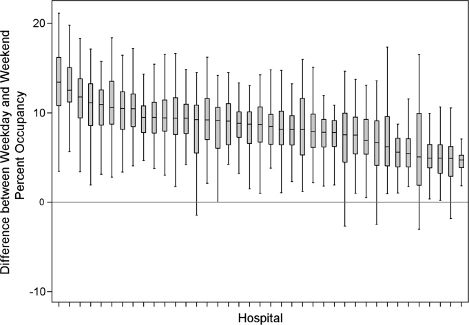
The characteristics of the 39 hospitals are provided in Table 1. Based on standardization with KID, 23.6% of PHIS admissions were scheduled (range: 18.1%35.8%) or a median of 81.5 scheduled admissions per week per hospital; 26.6% of weekday admissions were scheduled versus 16.1% for weekends. Overall, 12.4% of scheduled admissions entered on weekends. For all patients, median LOS was three days (interquartile range [IQR]: twofive days), but median LOS for scheduled admissions was two days (IQR: onefour days). The median LOS and IQR were the same by day of admission for all days of the week. Most hospitals had an overall SLOSR close to one (median: 0.9, IQR: 0.91.1). Overall, hospital mean midnight occupancy ranged from 70.9% to 108.1% on weekdays and 65.7% to 94.9% on weekends. Uniformly, weekday occupancy exceeded weekend occupancy, with a median difference of 8.2% points (IQR: 7.2%9.5% points). There was a wide range of median hospital weekdayweekend occupancy differences across hospitals (Figure 1). The overall difference was less in winter (median difference: 7.7% points; IQR: 6.3%8.8% points) than in summer (median difference: 8.6% points; IQR: 7.4%9.8% points (Wilcoxon Sign Rank test, P < 0.001). Thirty‐five hospitals (89.7%) exceeded the 85% occupancy threshold and 29 (74.4%) exceeded the 95% occupancy threshold on at least 20% of weekdays (Table 2). Across all the hospitals, the median difference in weekly maximum and weekly mean occupancy was 6.6% points (IQR: 6.2%7.4% points) (Figure 2).
| Characteristics | No. (%) |
|---|---|
| |
| Licensed in‐service beds | n = 39 hospitals |
| <200 beds | 6 (15.4) |
| 200249 beds | 10 (25.6) |
| 250300 beds | 14 (35.9) |
| >300 beds | 9 (23.1) |
| No. of discharges | |
| <10,000 | 5 (12.8) |
| 10,00013,999 | 14 (35.9) |
| 14,00017,999 | 11 (28.2) |
| >18,000 | 9 (23.1) |
| Census region | |
| West | 9 (23.1) |
| Midwest | 11 (28.2) |
| Northeast | 6 (15.4) |
| South | 13 (33.3) |
| Admissions | n = 590,352 admissions |
| Medical scheduled admissions* | 79,683 |
| Surgical scheduled admissions* | 59,640 |
| Total scheduled admissions* (% of all admissions) | 139,323 (23.6) |
| Weekend medical scheduled admissions* (% of all medical scheduled admissions) | 13,546 (17.0) |
| Weekend surgical scheduled admissions* (% of all surgical scheduled admissions) | 3,757 (6.3) |
| Weekend total scheduled admissions* (% of total scheduled admissions) | 17,276 (12.4) |

| Entire Year | >85% | Occupancy Threshold | >95% | >100% |
|---|---|---|---|---|
| >90% | ||||
| ||||
| No. of hospitals (n = 39) with mean weekday occupancy above threshold | ||||
| Before smoothing (current state) | 33 | 25 | 14 | 6 |
| After smoothing | 32 | 22 | 10 | 1 |
| No. of hospitals (n = 39) above threshold 20% of weekdays | ||||
| Before smoothing (current state) | 35 | 34 | 29 | 14 |
| After smoothing | 35 | 32 | 21 | 9 |
| Median (IQR) no. of patient‐days per hospital not exposed to occupancy above threshold by smoothing | 3,071 | 281 | 3236 | 3281 |
| (5,552, 919) | (5,288, 3,103) | (0, 7,083) | (962, 8,517) | |
| Median (IQR) no. of patients per hospital not exposed to occupancy above threshold by smoothing | 596 | 50 | 630 | 804 |
| (1,190, 226) | (916, 752) | (0, 1,492) | (231, 2,195) | |
Smoothing reduced the number of hospitals at each occupancy threshold, except 85% (Table 2). As a linear relationship, the reduction in weekday peak occupancy (y) based on a hospital's median difference in weekly maximum and weekly mean occupancy (x) was y = 2.69 + 0.48x. Thus, a hospital with a 10% point difference between weekday and weekend occupancy could reduce weekday peak by 7.5% points.
Smoothing increased the number of patients exposed to the lower thresholds (85% and 90%), but decreased the number of patients exposed to >95% occupancy (Table 2). For example, smoothing at the 95% threshold resulted in 630 fewer patients per hospital exposed to that threshold. If all 39 hospitals had within‐week smoothing, a net of 39,607 patients would have been protected from exposure to >95% occupancy and a net of 50,079 patients from 100% occupancy.
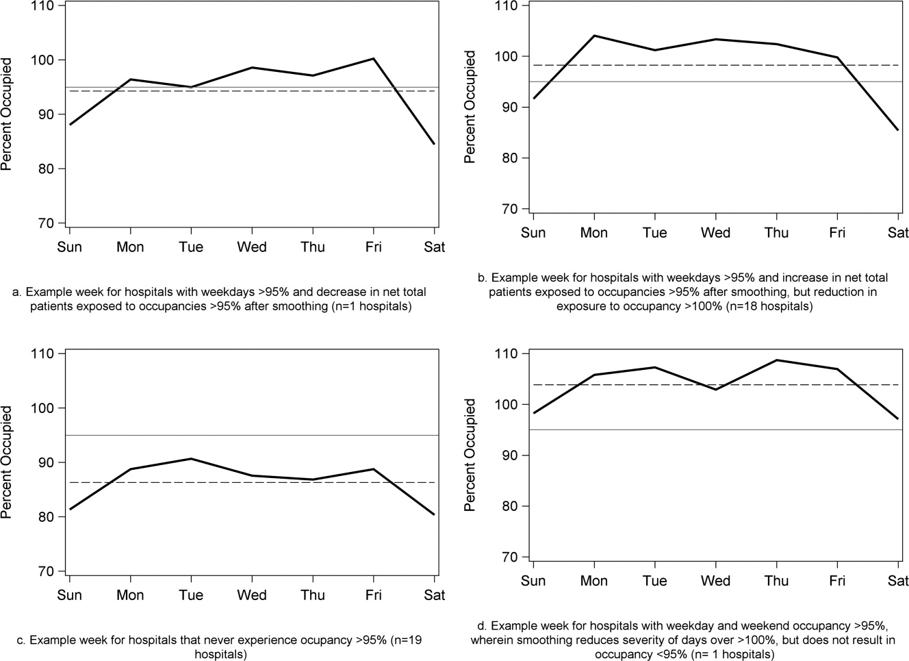
To demonstrate the varied effects of smoothing, Table 3 and Figure 3 present representative categories of response to smoothing depending on pre‐smoothing patterns. While not all hospitals decreased occupancy to below thresholds after smoothing (Types B and D), the overall occupancy was reduced and fewer patients were exposed to extreme levels of high occupancy (eg, >100%).
| Category | Before Smoothing Hospital Description | After Smoothing Hospital Description | No. of Hospitals at 85% Threshold (n = 39) | No. of Hospitals at 95% Threshold (n = 39) |
|---|---|---|---|---|
| ||||
| Type A | Weekdays above threshold | All days below threshold, resulting in net decrease in patients exposed to occupancies above threshold | 3 | 1 |
| Weekends below threshold | ||||
| Type B | Weekdays above threshold | All days above threshold, resulting in net increase in patients exposed to occupancies above threshold | 12 | 18 |
| Weekends below threshold | ||||
| Type C | All days of week below threshold | All days of week below threshold | 6 | 19 |
| Type D | All days of week above threshold | All days of week above threshold, resulting in net decrease in patients exposed to extreme high occupancy | 18 | 1 |
To achieve within‐week smoothing, a median of 7.4 patient‐admissions per week (range: 2.314.4) would have to be scheduled on a different day of the week. This equates to a median of 2.6% (IQR: 2.25%, 2.99%; range: 0.02%9.2%) of all admissionsor 9% of a typical hospital‐week's scheduled admissions.
Discussion
This analysis of 39 children's hospitals found high levels of occupancy and weekend occupancy lower than weekday occupancy (median difference: 8.2% points). Only 12.4% of scheduled admissions entered on weekends. Thus, weekend capacity is available to offset high weekday occupancy. Hospitals at the higher end of the occupancy thresholds (95%, 100%) would reduce the number of days operating at very high occupancy and the number of patients exposed to such levels by smoothing. This change is mathematically feasible, as a median of 7.4 patients would have to be proactively scheduled differently each week, just under one‐tenth of scheduled admissions. Since LOS by day of admission was the same (median: two days), the opportunity to affect occupancy by shifting patients should be relatively similar for all days of the week. In addition, these admissions were short, conferring greater flexibility. Implementing smoothing over the course of the week does not necessarily require admitting patients on weekends. For example, Monday admissions with an anticipated three‐day LOS could enter on Friday with anticipated discharge on Monday to alleviate midweek crowding and take advantage of unoccupied weekend beds. 26
At the highest levels of occupancy, smoothing reduces the frequency of reaching these maximum levels, but can have the effect of actually exposing more patient‐days to a higher occupancy. For example, for nine hospitals in our analysis with >20% of days over 100%, smoothing decreased days over 100%, but exposed weekend patients to higher levels of occupancy (Figure 3). Since most admissions are short and most scheduled admissions currently occur on weekdays, the number of individual patients (not patient‐days) newly exposed to such high occupancy may not increase much after smoothing at these facilities. Regardless, hospitals with such a pattern may not be able to rely solely on smoothing to avoid weekday crowding, and, if they are operating efficiently in terms of SLOSR, might be justified in building more capacity.
Consistent with our findings, the Institute for Healthcare Improvement, the Institute for Healthcare Optimization, and the American Hospital Association Quality Center stress that addressing artificial variability of scheduled admissions is a critical first step to improving patient flow and quality of care while reducing costs. 18, 21, 27 Our study suggests that small numbers of patients need to be proactively scheduled differently to decrease midweek peak occupancy, so only a small proportion of families would need to find this desirable to make it attractive for hospitals and patients. This type of proactive smoothing decreases peak occupancy on weekdays, reducing the safety risks associated with high occupancy, improving acute access for emergent patients, shortening wait‐times and loss of scheduled patients to another facility, and increasing procedure volume (3%74% in one study). 28 Smoothing may also increase quality and safety on weekends, as emergent patients admitted on weekends experience more delays in necessary treatment and have worse outcomes. 2932 In addition, increasing scheduled admissions to span weekends may appeal to some families wishing to avoid absence from work to be with their hospitalized child, to parents concerned about school performanceand may also appeal to staff members seeking flexible schedules. Increasing weekend hospital capacity is safe, feasible, and economical, even when considering the increased wages for weekend work. 33, 34 Finally, smoothing over the whole week allows fixed costs (eg, surgical suites, imaging equipment) to be allocated over 7 days rather than 5, and allows for better matching of revenue to the fixed expenses.
Rather than a prescriptive approach, our work suggests hospitals need to identify only a small number of patients to proactively shift, providing them opportunities to adapt the approach to local circumstances. The particular patients to move around may also depend on the costs and benefits of services (eg, radiologic, laboratory, operative) and the hospital's existing patterns of staffing. A number of hospitals that have engaged in similar work have achieved sustainable results, such as Seattle Children's Hospital, Boston Medical Center, St. John's Regional Health Center, and New York University Langone Medical Center. 19, 26, 3537 In these cases, proactive smoothing took advantage of unused capacity and decreased crowding on days that had been traditionally very full. Hospitals that rarely or never have high‐occupancy days, and that do not expect growth in volume, may not need to employ smoothing, whereas others that have crowding issues primarily in the winter may wish to implement smoothing techniques seasonally.
Aside from attempting to reduce high‐occupancy through modification of admission patterns, other proactive approaches include optimizing staffing and processes around care, improving efficiency of care, and building additional beds. 16, 25, 38, 39 However, the expense of construction and the scarcity of capital often preclude this last option. Among children's hospitals, with SLOSR close to one, implementing strategies to reduce the LOS during periods of high occupancy may not result in meaningful reductions in LOS, as such approaches would only decrease the typical child's hospitalization by hours, not days. In addition to proactive strategies, hospitals also rely on reactive approaches, such as ED boarding, placing patients in hallways on units, diverting ambulances or transfers, or canceling scheduled admissions at the last moment, to decrease crowding. 16, 39, 40
This study has several limitations. First, use of administrative data precluded modeling all responses. For example, some hospitals may be better able to accommodate fluctuations in census or high occupancy without compromising quality or access. Second, we only considered intra‐week smoothing, but hospitals may benefit from smoothing over longer periods of time, especially since children's hospitals are busier in winter months, but incoming scheduled volume is often not reduced. 11 Hospitals with large occupancy variations across months may want to consider broadening the time horizon for smoothing, and weigh the costs and benefits over that period of time, including parental and clinician concerns and preferences for not delaying treatment. At the individual hospital level, discrete‐event simulation would likely be useful to consider the trade‐offs of smoothing to different levels and over different periods of time. Third, we assumed a fixed number of beds for the year, an approach that may not accurately reflect actual available beds on specific days. This limitation was minimized by counting all beds for each hospital as available for all the days of the year, so that hospitals with a high census when all available beds are included would have an even higher percent occupancy if some of those beds were not actually open. In a related way, then, we also do not consider how staffing may need to be altered or augmented to care for additional patients on certain days. Fourth, midnight census, the only universally available measure, was used to determine occupancy rather than peak census. Midnight census provides a standard snapshot, but is lower than mid‐day peak census. 41 In order to account for these limitations, we considered several different thresholds of high occupancy. Fifth, we smoothed at the hospital level, but differential effects may exist at the unit level. Sixth, to determine proportion of scheduled admissions, we used HCUP KID proportions on PHIS admissions. Overall, this approach likely overestimated scheduled medical admissions on weekends, thus biasing our result towards the null hypothesis. Finally, only freestanding children's hospitals were included in this study. While this may limit generalizability, the general concept of smoothing occupancy should apply in any setting with substantial and consistent variation.
In summary, our study revealed that children's hospitals often face high midweek occupancy, but also have substantial unused weekend capacity. Hospitals facing challenges with high weekday occupancy could proactively use a smoothing approach to decrease the frequency and severity of high occupancy. Further qualitative evaluation is also warranted around child, family, and staff preferences concerning scheduled admissions, school, and work.
- , , , . A comparison of in‐hospital mortality risk conferred by high hospital occupancy, differences in nurse staffing levels, weekend admission, and seasonal influenza. Medical Care. 2010;48(3):224–232.
- , , , et al. Hospital workload and adverse events. Med Care. 2007;45(5):448–455.
- , , , , . Impact of admission‐day crowding on the length of stay of pediatric hospitalizations. Pediatrics. 2008;121(4):e718–e730.
- , , , . The effect of hospital bed occupancy on throughput in the pediatric emergency department. Ann Emerg Med. 2009;53(6):767–776.
- . The tipping point: the relationship between volume and patient harm. Am J Med Qual. 2008;23(5):336–341.
- , , , , , . Managing unnecessary variability in patient demand to reduce nursing stress and improve patient safety. Jt Comm J Qual Patient Saf. 2005;31(6):330–338.
- Hospital‐Based Emergency Care: At the Breaking Point. Washington, DC: Institute of Medicine Committee on the Future of Emergency Care in the United States Health System; 2006.
- , , , , . The effect of hospital occupancy on emergency department length of stay and patient disposition. Acad Emerg Med. 2003;10(2):127–133.
- . Interpreting the Volume‐Outcome Relationship in the Context of Health Care Quality: Workshop Summary. Washington, DC: National Academies Press; 2000.
- , , , , . Has recognition of the relationship between mortality rates and hospital volume for major cancer surgery in California made a difference? A follow‐up analysis of another decade. Ann Surg. 2009;250(3):472–483.
- , , , et al. Children's hospitals do not acutely respond to high occupancy. Pediatrics. 2010;125:974–981.
- , , , , , . Scheduled admissions and high occupancy at a children's hospital. J Hosp Med. 2011;6(2):81–87.
- , , . Characteristics of weekday and weekend hospital admissions. HCUP Statistical Brief. 2010;87.
- Agency for Healthcare Research and Quality. HCUP databases, Healthcare Cost and Utilization Project (HCUP); 2008. Available at: http://www.hcup‐us.ahrq.gov/kidoverview.jsp. Accessed July 15, 2009.
- , et al. Managing capacity to reduce emergency department overcrowding and ambulance diversions. J Qual Patient Saf. 2006;32(5):239–245.
- Institute for Healthcare Improvement. Flow initiatives; 2008. Available at: http://www.ihi.org/IHI/Topics/Flow. Accessed February 20, 2008.
- , , , , , . Trends in high‐turnover stays among children hospitalized in the United States, 1993–2003. Pediatrics. 2009;123(3):996–1002.
- Institute for Healthcare Improvement. Smoothing elective surgical admissions. Available at: http://www.ihi.org/IHI/Topics/Flow/PatientFlow/EmergingContent/SmoothingElectiveSurgicalAdmissions.htm. Accessed October 24, 2008.
- Boston hospital sees big impact from smoothing elective schedule. OR Manager. 2004;20:12.
- . Managing Variability in Patient Flow Is the Key to Improving Access to Care, Nursing Staffing, Quality of Care, and Reducing Its Cost. Paper presented at Institute of Medicine, Washington, DC; June 24, 2004.
- American Hospital Association Quality Center. Available at: http://www.ahaqualitycenter.org/ahaqualitycenter/. Accessed October 14, 2008.
- Healthcare Cost and Utilization Project (HCUP). Kids' Inpatient Database (KID); July 2008. Available at: http://www.hcup‐us.ahrq.gov/kidoverview.jsp. Accessed September 10, 2008.
- , , . Using a queuing model to help plan bed allocation in a department of geriatric medicine. Health Care Manag Sci. 2002;5(4):307–313.
- . How many hospital beds? Inquiry. 2002;39(4):400–412.
- . Institute for Healthcare Improvement. Patient flow comments. Available at: http://www.ihi.org/IHI/Topics/Flow. Accessed September 10, 2008.
- . Factory efficiency comes to the hospital. New York Times. July 9, 2010.
- Institute for Healthcare Improvement. Re‐engineering the operating room. Available at: http://www.ihi.org/IHI/Programs/ConferencesAndSeminars/ReengineeringtheOperatingRoomSept08.htm. Accessed November 8, 2008.
- , . Enhanced weekend service: an affordable means to increased hospital procedure volume. CMAJ. 2005;172(4):503–504.
- , . Mortality among patients admitted to hospitals on weekends as compared with weekdays. N Engl J Med. 2001;345:663–668.
- , , , , , . Weekend versus weekday admission and mortality from myocardial infarction. N Engl J Med. 2007;356:1099–1109.
- , . Waiting for urgent procedures on the weekend among emergently hospitalized patients. Am J Med. 2004;117:175–181.
- . Do hospitals provide lower quality care on weekends? Health Serv Res. 2007;42:1589–1612.
- . Hospital saves by working weekends. Mod Healthc. 1996;26:82–99.
- , , , , . Weekend and holiday exercise testing in patients with chest pain. J Gen Intern Med. 1999;14:10–14.
- . Boston Medical Center Case Study: Institute of Healthcare Optimization; 2006. Available at: http://www.ihoptimize.org/8f16e142‐eeaa‐4898–9e62–660218f19ffb/download.htm. Accessed October 3, 2010.
- , , , . The impact of IMPACT on St John's Regional Health Center. Mo Med. 2003;100:590–592.
- NYU Langone Medical Center Extends Access to Non‐Emergent Care as Part of Commitment to Patient‐Centered Care (June 23, 2010). Available at: http://communications.med.nyu.edu/news/2010/nyu‐langone‐medical‐center‐extends‐access‐non‐emergent‐care‐part‐commitment‐patient‐center. Accessed October 3, 2010.
- Carondelet St. Mary's Hospital. A pragmatic approach to improving patient efficiency throughput. Improvement Report 2005. Available at: http://www.ihi.org/IHI/Topics/Flow/PatientFlow/ImprovementStories/APragmaticApproachtoImprovingPatientEfficiencyThroughput.htm. Accessed October 3, 2010.
- AHA Solutions. Patient Flow Challenges Assessment 2009. Chicago, IL; 2009.
- , , , , , . A conceptual model of emergency department crowding. Ann Emerg Med. 2003;42(2):173–180.
- . Annual bed statistics give a misleading picture of hospital surge capacity. Ann Emerg Med. 2006;48(4):384–388.
High levels of hospital occupancy are associated with compromises to quality of care and access (often referred to as crowding), 18 while low occupancy may be inefficient and also impact quality. 9, 10 Despite this, hospitals typically have uneven occupancy. Although some demand for services is driven by factors beyond the control of a hospital (eg, seasonal variation in viral illness), approximately 15%30% of admissions to children's hospitals are scheduled from days to months in advance, with usual arrivals on weekdays. 1114 For example, of the 3.4 million elective admissions in the 2006 Healthcare Cost and Utilization Project Kids Inpatient Database (HCUP KID), only 13% were admitted on weekends. 14 Combined with short length of stay (LOS) for such patients, this leads to higher midweek and lower weekend occupancy. 12
Hospitals respond to crowding in a number of ways, but often focus on reducing LOS to make room for new patients. 11, 15, 16 For hospitals that are relatively efficient in terms of LOS, efforts to reduce it may not increase functional capacity adequately. In children's hospitals, median lengths of stay are 2 to 3 days, and one‐third of hospitalizations are 1 day or less. 17 Thus, even 10%20% reductions in LOS trims hours, not days, from typical stays. Practical barriers (eg, reluctance to discharge in the middle of the night, or family preferences and work schedules) and undesired outcomes (eg, increased hospital re‐visits) are additional pitfalls encountered by relying on throughput enhancement alone.
Managing scheduled admissions through smoothing is an alternative strategy to reduce variability and high occupancy. 6, 12, 1820 The concept is to proactively control the entry of patients, when possible, to achieve more even levels of occupancy, instead of the peaks and troughs commonly encountered. Nonetheless, it is not a widely used approach. 18, 20, 21 We hypothesized that children's hospitals had substantial unused capacity that could be used to smooth occupancy, which would reduce weekday crowding. While it is obvious that smoothing will reduce peaks to average levels (and also raise troughs), we sought to quantify just how large this difference wasand thereby quantify the potential of smoothing to reduce inpatient crowding (or, conversely, expose more patients to high levels of occupancy). Is there enough variation to justify smoothing, and, if a hospital does smooth, what is the expected result? If the number of patients removed from exposure to high occupancy is not substantial, other means to address inpatient crowding might be of more value. Our aims were to quantify the difference in weekday versus weekend occupancy, report on mathematical feasibility of such an approach, and determine the difference in number of patients exposed to various levels of high occupancy.
Methods
Data Source
This retrospective study was conducted with resource‐utilization data from 39 freestanding, tertiary‐care children's hospitals in the Pediatric Health Information System (PHIS). Participating hospitals are located in noncompeting markets of 23 states, plus the District of Columbia, and affiliated with the Child Health Corporation of America (CHCA, Shawnee Mission, KS). They account for 80% of freestanding, and 20% of all general, tertiary‐care children's hospitals. Data quality and reliability are assured through joint ongoing, systematic monitoring. The Children's Hospital of Philadelphia Committees for the Protection of Human Subjects approved the protocol with a waiver of informed consent.
Patients
Patients admitted January 1December 31, 2007 were eligible for inclusion. Due to variation in the presence of birthing, neonatal intensive care, and behavioral health units across hospitals, these beds and associated patients were excluded. Inpatients enter hospitals either as scheduled (often referred to as elective) or unscheduled (emergent or urgent) admissions. Because PHIS does not include these data, KID was used to standardize the PHIS data for proportion of scheduled admissions. 22 (KID is a healthcare database of 23 million pediatric inpatient discharges developed through federalstateindustry partnership, and sponsored by the Agency for Healthcare Research and Quality [AHRQ].) Each encounter in KID includes a principal International Classification of Diseases, 9th revision (ICD‐9) discharge diagnosis code, and is designated by the hospital as elective (ranging from chemotherapy to tonsillectomy) or not elective. Because admissions, rather than diagnoses, are scheduled, a proportion of patients with each primary diagnosis in KID are scheduled (eg, 28% of patients with a primary diagnosis of esophageal reflux). Proportions in KID were matched to principal diagnoses in PHIS.
Definitions
The census was the number of patients registered as inpatients (including those physically in the emergency department [ED] from time of ED arrival)whether observation or inpatient statusat midnight, the conclusion of the day. Hospital capacity was set using CHCA data (and confirmed by each hospital's administrative personnel) as the number of licensed in‐service beds available for patients in 2007; we assumed beds were staffed and capacity fixed for the year. Occupancy was calculated by dividing census by capacity. Maximum occupancy in a week referred to the highest occupancy level achieved in a seven‐day period (MondaySunday). We analyzed a set of thresholds for high‐occupancy (85%, 90%, 95%, and 100%), because there is no consistent definition for when hospitals are at high occupancy or when crowding occurs, though crowding has been described as starting at 85% occupancy. 2325
Analysis
The hospital was the unit of analysis. We report hospital characteristics, including capacity, number of discharges, and census region, and annual standardized length of stay ratio (SLOSR) as observed‐to‐expected LOS.
Smoothing Technique
A retrospective smoothing algorithm set each hospital's daily occupancy during a week to that hospital's mean occupancy for the week; effectively spreading the week's volume of patients evenly across the days of the week. While inter‐week and inter‐month smoothing were considered, intra‐week smoothing was deemed more practical for the largest number of patients, as it would not mean delaying care by more than one week. In the case of a planned treatment course (eg, chemotherapy), only intra‐week smoothing would maintain the necessary scheduled intervals of treatment.
Mathematical Feasibility
To approximate the number of patient admissions that would require different scheduling during a particular week to achieve smoothed weekly occupancy, we determined the total number of patient‐days in the week that required different scheduling and divided by the average LOS for the week. We then divided the number of admissions‐to‐move by total weekly admissions to compute the percentage at each hospital across 52 weeks of the year.
Measuring the Impact of Smoothing
We focused on the frequency and severity of high occupancy and the number of patients exposed to it. This framework led to 4 measures that assess the opportunity and effect of smoothing:
Difference in hospital weekdayweekend occupancy: Equal to 12‐month median of difference between mean weekday occupancy and mean weekend occupancy for each hospital‐week.
Difference in hospital maximummean occupancy: Equal to median of difference between maximum one‐day occupancy and weekly mean (smoothed) occupancy for each hospital‐week. A regression line was derived from the data for the 39 hospitals to report expected reduction in peak occupancy based on the magnitude of the difference between weekday and weekend occupancy.
Difference in number of hospitals exposed to above‐threshold occupancy: Equal to difference, pre‐ and post‐smoothing, in number of hospitals facing high‐occupancy conditions on an average of at least one weekday midnight per week during the year at different occupancy thresholds.
Difference in number of patients exposed to above‐threshold occupancy: Equal to difference, pre‐ and post‐smoothing, in number of patients exposed to hospital midnight occupancy at the thresholds. We utilized patient‐days for the calculation to avoid double‐counting, and divided this by average LOS, in order to determine the number of patients who would no longer be exposed to over‐threshold occupancy after smoothing, while also adjusting for patients newly exposed to over‐threshold occupancy levels.
All analyses were performed separately for each hospital for the entire year and then for winter (DecemberMarch), the period during which most crowding occurred. Analyses were performed using SAS (version 9.2, SAS Institute, Inc, Cary, NC); P values <0.05 were considered statistically significant.
Results
The characteristics of the 39 hospitals are provided in Table 1. Based on standardization with KID, 23.6% of PHIS admissions were scheduled (range: 18.1%35.8%) or a median of 81.5 scheduled admissions per week per hospital; 26.6% of weekday admissions were scheduled versus 16.1% for weekends. Overall, 12.4% of scheduled admissions entered on weekends. For all patients, median LOS was three days (interquartile range [IQR]: twofive days), but median LOS for scheduled admissions was two days (IQR: onefour days). The median LOS and IQR were the same by day of admission for all days of the week. Most hospitals had an overall SLOSR close to one (median: 0.9, IQR: 0.91.1). Overall, hospital mean midnight occupancy ranged from 70.9% to 108.1% on weekdays and 65.7% to 94.9% on weekends. Uniformly, weekday occupancy exceeded weekend occupancy, with a median difference of 8.2% points (IQR: 7.2%9.5% points). There was a wide range of median hospital weekdayweekend occupancy differences across hospitals (Figure 1). The overall difference was less in winter (median difference: 7.7% points; IQR: 6.3%8.8% points) than in summer (median difference: 8.6% points; IQR: 7.4%9.8% points (Wilcoxon Sign Rank test, P < 0.001). Thirty‐five hospitals (89.7%) exceeded the 85% occupancy threshold and 29 (74.4%) exceeded the 95% occupancy threshold on at least 20% of weekdays (Table 2). Across all the hospitals, the median difference in weekly maximum and weekly mean occupancy was 6.6% points (IQR: 6.2%7.4% points) (Figure 2).
| Characteristics | No. (%) |
|---|---|
| |
| Licensed in‐service beds | n = 39 hospitals |
| <200 beds | 6 (15.4) |
| 200249 beds | 10 (25.6) |
| 250300 beds | 14 (35.9) |
| >300 beds | 9 (23.1) |
| No. of discharges | |
| <10,000 | 5 (12.8) |
| 10,00013,999 | 14 (35.9) |
| 14,00017,999 | 11 (28.2) |
| >18,000 | 9 (23.1) |
| Census region | |
| West | 9 (23.1) |
| Midwest | 11 (28.2) |
| Northeast | 6 (15.4) |
| South | 13 (33.3) |
| Admissions | n = 590,352 admissions |
| Medical scheduled admissions* | 79,683 |
| Surgical scheduled admissions* | 59,640 |
| Total scheduled admissions* (% of all admissions) | 139,323 (23.6) |
| Weekend medical scheduled admissions* (% of all medical scheduled admissions) | 13,546 (17.0) |
| Weekend surgical scheduled admissions* (% of all surgical scheduled admissions) | 3,757 (6.3) |
| Weekend total scheduled admissions* (% of total scheduled admissions) | 17,276 (12.4) |
| Entire Year | >85% | Occupancy Threshold | >95% | >100% |
|---|---|---|---|---|
| >90% | ||||
| ||||
| No. of hospitals (n = 39) with mean weekday occupancy above threshold | ||||
| Before smoothing (current state) | 33 | 25 | 14 | 6 |
| After smoothing | 32 | 22 | 10 | 1 |
| No. of hospitals (n = 39) above threshold 20% of weekdays | ||||
| Before smoothing (current state) | 35 | 34 | 29 | 14 |
| After smoothing | 35 | 32 | 21 | 9 |
| Median (IQR) no. of patient‐days per hospital not exposed to occupancy above threshold by smoothing | 3,071 | 281 | 3236 | 3281 |
| (5,552, 919) | (5,288, 3,103) | (0, 7,083) | (962, 8,517) | |
| Median (IQR) no. of patients per hospital not exposed to occupancy above threshold by smoothing | 596 | 50 | 630 | 804 |
| (1,190, 226) | (916, 752) | (0, 1,492) | (231, 2,195) | |
Smoothing reduced the number of hospitals at each occupancy threshold, except 85% (Table 2). As a linear relationship, the reduction in weekday peak occupancy (y) based on a hospital's median difference in weekly maximum and weekly mean occupancy (x) was y = 2.69 + 0.48x. Thus, a hospital with a 10% point difference between weekday and weekend occupancy could reduce weekday peak by 7.5% points.
Smoothing increased the number of patients exposed to the lower thresholds (85% and 90%), but decreased the number of patients exposed to >95% occupancy (Table 2). For example, smoothing at the 95% threshold resulted in 630 fewer patients per hospital exposed to that threshold. If all 39 hospitals had within‐week smoothing, a net of 39,607 patients would have been protected from exposure to >95% occupancy and a net of 50,079 patients from 100% occupancy.
To demonstrate the varied effects of smoothing, Table 3 and Figure 3 present representative categories of response to smoothing depending on pre‐smoothing patterns. While not all hospitals decreased occupancy to below thresholds after smoothing (Types B and D), the overall occupancy was reduced and fewer patients were exposed to extreme levels of high occupancy (eg, >100%).
| Category | Before Smoothing Hospital Description | After Smoothing Hospital Description | No. of Hospitals at 85% Threshold (n = 39) | No. of Hospitals at 95% Threshold (n = 39) |
|---|---|---|---|---|
| ||||
| Type A | Weekdays above threshold | All days below threshold, resulting in net decrease in patients exposed to occupancies above threshold | 3 | 1 |
| Weekends below threshold | ||||
| Type B | Weekdays above threshold | All days above threshold, resulting in net increase in patients exposed to occupancies above threshold | 12 | 18 |
| Weekends below threshold | ||||
| Type C | All days of week below threshold | All days of week below threshold | 6 | 19 |
| Type D | All days of week above threshold | All days of week above threshold, resulting in net decrease in patients exposed to extreme high occupancy | 18 | 1 |
To achieve within‐week smoothing, a median of 7.4 patient‐admissions per week (range: 2.314.4) would have to be scheduled on a different day of the week. This equates to a median of 2.6% (IQR: 2.25%, 2.99%; range: 0.02%9.2%) of all admissionsor 9% of a typical hospital‐week's scheduled admissions.
Discussion
This analysis of 39 children's hospitals found high levels of occupancy and weekend occupancy lower than weekday occupancy (median difference: 8.2% points). Only 12.4% of scheduled admissions entered on weekends. Thus, weekend capacity is available to offset high weekday occupancy. Hospitals at the higher end of the occupancy thresholds (95%, 100%) would reduce the number of days operating at very high occupancy and the number of patients exposed to such levels by smoothing. This change is mathematically feasible, as a median of 7.4 patients would have to be proactively scheduled differently each week, just under one‐tenth of scheduled admissions. Since LOS by day of admission was the same (median: two days), the opportunity to affect occupancy by shifting patients should be relatively similar for all days of the week. In addition, these admissions were short, conferring greater flexibility. Implementing smoothing over the course of the week does not necessarily require admitting patients on weekends. For example, Monday admissions with an anticipated three‐day LOS could enter on Friday with anticipated discharge on Monday to alleviate midweek crowding and take advantage of unoccupied weekend beds. 26
At the highest levels of occupancy, smoothing reduces the frequency of reaching these maximum levels, but can have the effect of actually exposing more patient‐days to a higher occupancy. For example, for nine hospitals in our analysis with >20% of days over 100%, smoothing decreased days over 100%, but exposed weekend patients to higher levels of occupancy (Figure 3). Since most admissions are short and most scheduled admissions currently occur on weekdays, the number of individual patients (not patient‐days) newly exposed to such high occupancy may not increase much after smoothing at these facilities. Regardless, hospitals with such a pattern may not be able to rely solely on smoothing to avoid weekday crowding, and, if they are operating efficiently in terms of SLOSR, might be justified in building more capacity.
Consistent with our findings, the Institute for Healthcare Improvement, the Institute for Healthcare Optimization, and the American Hospital Association Quality Center stress that addressing artificial variability of scheduled admissions is a critical first step to improving patient flow and quality of care while reducing costs. 18, 21, 27 Our study suggests that small numbers of patients need to be proactively scheduled differently to decrease midweek peak occupancy, so only a small proportion of families would need to find this desirable to make it attractive for hospitals and patients. This type of proactive smoothing decreases peak occupancy on weekdays, reducing the safety risks associated with high occupancy, improving acute access for emergent patients, shortening wait‐times and loss of scheduled patients to another facility, and increasing procedure volume (3%74% in one study). 28 Smoothing may also increase quality and safety on weekends, as emergent patients admitted on weekends experience more delays in necessary treatment and have worse outcomes. 2932 In addition, increasing scheduled admissions to span weekends may appeal to some families wishing to avoid absence from work to be with their hospitalized child, to parents concerned about school performanceand may also appeal to staff members seeking flexible schedules. Increasing weekend hospital capacity is safe, feasible, and economical, even when considering the increased wages for weekend work. 33, 34 Finally, smoothing over the whole week allows fixed costs (eg, surgical suites, imaging equipment) to be allocated over 7 days rather than 5, and allows for better matching of revenue to the fixed expenses.
Rather than a prescriptive approach, our work suggests hospitals need to identify only a small number of patients to proactively shift, providing them opportunities to adapt the approach to local circumstances. The particular patients to move around may also depend on the costs and benefits of services (eg, radiologic, laboratory, operative) and the hospital's existing patterns of staffing. A number of hospitals that have engaged in similar work have achieved sustainable results, such as Seattle Children's Hospital, Boston Medical Center, St. John's Regional Health Center, and New York University Langone Medical Center. 19, 26, 3537 In these cases, proactive smoothing took advantage of unused capacity and decreased crowding on days that had been traditionally very full. Hospitals that rarely or never have high‐occupancy days, and that do not expect growth in volume, may not need to employ smoothing, whereas others that have crowding issues primarily in the winter may wish to implement smoothing techniques seasonally.
Aside from attempting to reduce high‐occupancy through modification of admission patterns, other proactive approaches include optimizing staffing and processes around care, improving efficiency of care, and building additional beds. 16, 25, 38, 39 However, the expense of construction and the scarcity of capital often preclude this last option. Among children's hospitals, with SLOSR close to one, implementing strategies to reduce the LOS during periods of high occupancy may not result in meaningful reductions in LOS, as such approaches would only decrease the typical child's hospitalization by hours, not days. In addition to proactive strategies, hospitals also rely on reactive approaches, such as ED boarding, placing patients in hallways on units, diverting ambulances or transfers, or canceling scheduled admissions at the last moment, to decrease crowding. 16, 39, 40
This study has several limitations. First, use of administrative data precluded modeling all responses. For example, some hospitals may be better able to accommodate fluctuations in census or high occupancy without compromising quality or access. Second, we only considered intra‐week smoothing, but hospitals may benefit from smoothing over longer periods of time, especially since children's hospitals are busier in winter months, but incoming scheduled volume is often not reduced. 11 Hospitals with large occupancy variations across months may want to consider broadening the time horizon for smoothing, and weigh the costs and benefits over that period of time, including parental and clinician concerns and preferences for not delaying treatment. At the individual hospital level, discrete‐event simulation would likely be useful to consider the trade‐offs of smoothing to different levels and over different periods of time. Third, we assumed a fixed number of beds for the year, an approach that may not accurately reflect actual available beds on specific days. This limitation was minimized by counting all beds for each hospital as available for all the days of the year, so that hospitals with a high census when all available beds are included would have an even higher percent occupancy if some of those beds were not actually open. In a related way, then, we also do not consider how staffing may need to be altered or augmented to care for additional patients on certain days. Fourth, midnight census, the only universally available measure, was used to determine occupancy rather than peak census. Midnight census provides a standard snapshot, but is lower than mid‐day peak census. 41 In order to account for these limitations, we considered several different thresholds of high occupancy. Fifth, we smoothed at the hospital level, but differential effects may exist at the unit level. Sixth, to determine proportion of scheduled admissions, we used HCUP KID proportions on PHIS admissions. Overall, this approach likely overestimated scheduled medical admissions on weekends, thus biasing our result towards the null hypothesis. Finally, only freestanding children's hospitals were included in this study. While this may limit generalizability, the general concept of smoothing occupancy should apply in any setting with substantial and consistent variation.
In summary, our study revealed that children's hospitals often face high midweek occupancy, but also have substantial unused weekend capacity. Hospitals facing challenges with high weekday occupancy could proactively use a smoothing approach to decrease the frequency and severity of high occupancy. Further qualitative evaluation is also warranted around child, family, and staff preferences concerning scheduled admissions, school, and work.
- , , , . A comparison of in‐hospital mortality risk conferred by high hospital occupancy, differences in nurse staffing levels, weekend admission, and seasonal influenza. Medical Care. 2010;48(3):224–232.
- , , , et al. Hospital workload and adverse events. Med Care. 2007;45(5):448–455.
- , , , , . Impact of admission‐day crowding on the length of stay of pediatric hospitalizations. Pediatrics. 2008;121(4):e718–e730.
- , , , . The effect of hospital bed occupancy on throughput in the pediatric emergency department. Ann Emerg Med. 2009;53(6):767–776.
- . The tipping point: the relationship between volume and patient harm. Am J Med Qual. 2008;23(5):336–341.
- , , , , , . Managing unnecessary variability in patient demand to reduce nursing stress and improve patient safety. Jt Comm J Qual Patient Saf. 2005;31(6):330–338.
- Hospital‐Based Emergency Care: At the Breaking Point. Washington, DC: Institute of Medicine Committee on the Future of Emergency Care in the United States Health System; 2006.
- , , , , . The effect of hospital occupancy on emergency department length of stay and patient disposition. Acad Emerg Med. 2003;10(2):127–133.
- . Interpreting the Volume‐Outcome Relationship in the Context of Health Care Quality: Workshop Summary. Washington, DC: National Academies Press; 2000.
- , , , , . Has recognition of the relationship between mortality rates and hospital volume for major cancer surgery in California made a difference? A follow‐up analysis of another decade. Ann Surg. 2009;250(3):472–483.
- , , , et al. Children's hospitals do not acutely respond to high occupancy. Pediatrics. 2010;125:974–981.
- , , , , , . Scheduled admissions and high occupancy at a children's hospital. J Hosp Med. 2011;6(2):81–87.
- , , . Characteristics of weekday and weekend hospital admissions. HCUP Statistical Brief. 2010;87.
- Agency for Healthcare Research and Quality. HCUP databases, Healthcare Cost and Utilization Project (HCUP); 2008. Available at: http://www.hcup‐us.ahrq.gov/kidoverview.jsp. Accessed July 15, 2009.
- , et al. Managing capacity to reduce emergency department overcrowding and ambulance diversions. J Qual Patient Saf. 2006;32(5):239–245.
- Institute for Healthcare Improvement. Flow initiatives; 2008. Available at: http://www.ihi.org/IHI/Topics/Flow. Accessed February 20, 2008.
- , , , , , . Trends in high‐turnover stays among children hospitalized in the United States, 1993–2003. Pediatrics. 2009;123(3):996–1002.
- Institute for Healthcare Improvement. Smoothing elective surgical admissions. Available at: http://www.ihi.org/IHI/Topics/Flow/PatientFlow/EmergingContent/SmoothingElectiveSurgicalAdmissions.htm. Accessed October 24, 2008.
- Boston hospital sees big impact from smoothing elective schedule. OR Manager. 2004;20:12.
- . Managing Variability in Patient Flow Is the Key to Improving Access to Care, Nursing Staffing, Quality of Care, and Reducing Its Cost. Paper presented at Institute of Medicine, Washington, DC; June 24, 2004.
- American Hospital Association Quality Center. Available at: http://www.ahaqualitycenter.org/ahaqualitycenter/. Accessed October 14, 2008.
- Healthcare Cost and Utilization Project (HCUP). Kids' Inpatient Database (KID); July 2008. Available at: http://www.hcup‐us.ahrq.gov/kidoverview.jsp. Accessed September 10, 2008.
- , , . Using a queuing model to help plan bed allocation in a department of geriatric medicine. Health Care Manag Sci. 2002;5(4):307–313.
- . How many hospital beds? Inquiry. 2002;39(4):400–412.
- . Institute for Healthcare Improvement. Patient flow comments. Available at: http://www.ihi.org/IHI/Topics/Flow. Accessed September 10, 2008.
- . Factory efficiency comes to the hospital. New York Times. July 9, 2010.
- Institute for Healthcare Improvement. Re‐engineering the operating room. Available at: http://www.ihi.org/IHI/Programs/ConferencesAndSeminars/ReengineeringtheOperatingRoomSept08.htm. Accessed November 8, 2008.
- , . Enhanced weekend service: an affordable means to increased hospital procedure volume. CMAJ. 2005;172(4):503–504.
- , . Mortality among patients admitted to hospitals on weekends as compared with weekdays. N Engl J Med. 2001;345:663–668.
- , , , , , . Weekend versus weekday admission and mortality from myocardial infarction. N Engl J Med. 2007;356:1099–1109.
- , . Waiting for urgent procedures on the weekend among emergently hospitalized patients. Am J Med. 2004;117:175–181.
- . Do hospitals provide lower quality care on weekends? Health Serv Res. 2007;42:1589–1612.
- . Hospital saves by working weekends. Mod Healthc. 1996;26:82–99.
- , , , , . Weekend and holiday exercise testing in patients with chest pain. J Gen Intern Med. 1999;14:10–14.
- . Boston Medical Center Case Study: Institute of Healthcare Optimization; 2006. Available at: http://www.ihoptimize.org/8f16e142‐eeaa‐4898–9e62–660218f19ffb/download.htm. Accessed October 3, 2010.
- , , , . The impact of IMPACT on St John's Regional Health Center. Mo Med. 2003;100:590–592.
- NYU Langone Medical Center Extends Access to Non‐Emergent Care as Part of Commitment to Patient‐Centered Care (June 23, 2010). Available at: http://communications.med.nyu.edu/news/2010/nyu‐langone‐medical‐center‐extends‐access‐non‐emergent‐care‐part‐commitment‐patient‐center. Accessed October 3, 2010.
- Carondelet St. Mary's Hospital. A pragmatic approach to improving patient efficiency throughput. Improvement Report 2005. Available at: http://www.ihi.org/IHI/Topics/Flow/PatientFlow/ImprovementStories/APragmaticApproachtoImprovingPatientEfficiencyThroughput.htm. Accessed October 3, 2010.
- AHA Solutions. Patient Flow Challenges Assessment 2009. Chicago, IL; 2009.
- , , , , , . A conceptual model of emergency department crowding. Ann Emerg Med. 2003;42(2):173–180.
- . Annual bed statistics give a misleading picture of hospital surge capacity. Ann Emerg Med. 2006;48(4):384–388.
Copyright © 2011 Society of Hospital Medicine